The Weekend Quiz – September 8-9, 2018 – answers and discussion

Here are the answers with discussion for this Weekend’s Quiz. The information provided should help you work out why you missed a question or three! If you haven’t already done the Quiz from yesterday then have a go at it before you read the answers. I hope this helps you develop an understanding of Modern Monetary Theory (MMT) and its application to macroeconomic thinking. Comments as usual welcome, especially if I have made an error.

Question 1:

If yields rise on new bond issues then deficit spending by a currency-issuing government becomes more expensive.

The answer is False.

To say that government spending is becoming more expensive assumes that there is some revenue constraint on government spending. The interest servicing payments come from the same source as all government spending – its infinite (minus $1!) capacity to issue fiat currency.

The correct measure of the ‘cost’ (that is, expensiveness) of government spending (deficit or otherwise) is related to the real productive resources that the government brings into use as a result of its demand.

So when the government issues a new bond, there is no ‘cost’ in real terms incurred.

The concept of more or less expensive is therefore inapplicable to spending by a currency-issuing government.

Typically, rising bond yields in a growing economy signal a growing confidence among private investors.

In macroeconomics, we summarise the plethora of public debt instruments with the concept of a bond. The standard bond has a face value – say $A1000 and a coupon rate – say 5 per cent and a maturity – say 10 years. This means that the bond holder will will get $50 dollar per annum (interest) for 10 years and when the maturity is reached they would get $1000 back.

Bonds are issued by government into the primary market, which is simply the institutional machinery via which the government sells debt to “raise funds”. In a modern monetary system with flexible exchange rates it is clear the government does not have to finance its spending so the the institutional machinery is voluntary and reflects the prevailing neo-liberal ideology – which emphasises a fear of fiscal excesses rather than any intrinsic need.

Once bonds are issued they are traded in the secondary market between interested parties. Clearly secondary market trading has no impact at all on the volume of financial assets in the system – it just shuffles the wealth between wealth-holders. In the context of public debt issuance – the transactions in the primary market are vertical (net financial assets are created or destroyed) and the secondary market transactions are all horizontal (no new financial assets are created). Please read my blog – Deficit spending 101 – Part 3 – for more discussion on this point.

Further, most primary market issuance is now done via auction. Accordingly, the government would determine the maturity of the bond (how long the bond would exist for), the coupon rate (the interest return on the bond) and the volume (how many bonds) being specified.

The issue would then be put out for tender and the market then would determine the final price of the bonds issued. Imagine a $1000 bond had a coupon of 5 per cent, meaning that you would get $50 dollar per annum until the bond matured at which time you would get $1000 back.

Imagine that the market wanted a yield of 6 per cent to accommodate risk expectations (inflation or something else). So for them the bond is unattractive and they would avoid it under the tap system. But under the tender or auction system they would put in a purchase bid lower than the $1000 to ensure they get the 6 per cent return they sought.

The mathematical formulae to compute the desired (lower) price is quite tricky and you can look it up in a finance book.

The general rule for fixed-income bonds is that when the prices rise, the yield falls and vice versa. Thus, the price of a bond can change in the market place according to interest rate fluctuations.

When interest rates rise, the price of previously issued bonds fall because they are less attractive in comparison to the newly issued bonds, which are offering a higher coupon rates (reflecting current interest rates).

When interest rates fall, the price of older bonds increase, becoming more attractive as newly issued bonds offer a lower coupon rate than the older higher coupon rated bonds.

Further, rising yields may indicate a rising sense of risk (mostly from future inflation although sovereign credit ratings will influence this). But they may also indicated a recovering economy where people are more confidence investing in commercial paper (for higher returns) and so they demand less of the “risk free” government paper.

So you see how an event (yield rises) that signifies growing confidence in the real economy is reinterpreted (and trumpeted) by the conservatives to signal something bad (crowding out).

n this case, the reason long-term yields would be rising is because investors were diversifying their portfolios and moving back into private financial assets.

The yield reflects the last auction bid in the bond issue. So if diversification is occurring reflecting confidence and the demand for public debt weakens and yields rise this has nothing at all to do with a declining pool of funds being soaked up by the binging government!

The following blogs may be of further interest to you:

• Saturday Quiz – April 17, 2010 – answers and discussion
• Time to outlaw the credit rating agencies
• Studying macroeconomics – an exercise in deception
• Time for a reality check on debt – Part 1
• Will we really pay higher interest rates?

Question 2:

In a fiat monetary system (for example, US or Australia) with an on-going external deficit that exceeds the public deficit (expressed as percentages of GDP), the domestic private sector cannot reduce its overall debt levels (by overall saving) without incurring employment losses and pushing the public deficit higher and the external deficit lower.

The answer is True.

This question is an application of the sectoral balances framework that can be derived from the National Accounts for any nation.

To refresh your memory the balances are derived as follows. The basic income-expenditure model in macroeconomics can be viewed in (at least) two ways: (a) from the perspective of the sources of spending; and (b) from the perspective of the uses of the income produced. Bringing these two perspectives (of the same thing) together generates the sectoral balances.

From the sources perspective we write:

(1) GDP = C + I + G + (X – M)

which says that total national income (GDP) is the sum of total final consumption spending (C), total private investment (I), total government spending (G) and net exports (X – M).

Expression (1) tells us that total income in the economy per period will be exactly equal to total spending from all sources of expenditure.

We also have to acknowledge that financial balances of the sectors are impacted by net government taxes (T) which includes all tax revenue minus total transfer and interest payments (the latter are not counted independently in the expenditure Expression (1)).

Further, as noted above the trade account is only one aspect of the financial flows between the domestic economy and the external sector. we have to include net external income flows (FNI).

Adding in the net external income flows (FNI) to Expression (2) for GDP we get the familiar gross national product or gross national income measure (GNP):

(2) GNP = C + I + G + (X – M) + FNI

To render this approach into the sectoral balances form, we subtract total net taxes (T) from both sides of Expression (3) to get:

(3) GNP – T = C + I + G + (X – M) + FNI – T

Now we can collect the terms by arranging them according to the three sectoral balances:

(4) (GNP – C – T) – I = (G – T) + (X – M + FNI)

The the terms in Expression (4) are relatively easy to understand now.

The term (GNP – C – T) represents total income less the amount consumed less the amount paid to government in taxes (taking into account transfers coming the other way). In other words, it represents private domestic saving.

The left-hand side of Equation (4), (GNP – C – T) – I, thus is the overall saving of the private domestic sector, which is distinct from total household saving denoted by the term (GNP – C – T).

In other words, the left-hand side of Equation (4) is the private domestic financial balance and if it is positive then the sector is spending less than its total income and if it is negative the sector is spending more than it total income.

The term (G – T) is the government financial balance and is in deficit if government spending (G) is greater than government tax revenue minus transfers (T), and in surplus if the balance is negative.

Finally, the other right-hand side term (X – M + FNI) is the external financial balance, commonly known as the current account balance (CAD). It is in surplus if positive and deficit if negative.

In English we could say that:

The private financial balance equals the sum of the government financial balance plus the current account balance.

We can re-write Expression (6) in this way to get the sectoral balances equation:

(5) (S – I) = (G – T) + CAD

which is interpreted as meaning that government sector deficits (G – T > 0) and current account surpluses (CAD > 0) generate national income and net financial assets for the private domestic sector.

Conversely, government surpluses (G – T < 0) and current account deficits (CAD < 0) reduce national income and undermine the capacity of the private domestic sector to add financial assets.

Expression (5) can also be written as:

(6) [(S – I) – CAD] = (G – T)

where the term on the left-hand side [(S – I) – CAD] is the non-government sector financial balance and is of equal and opposite sign to the government financial balance.

This is the familiar MMT statement that a government sector deficit (surplus) is equal dollar-for-dollar to the non-government sector surplus (deficit).

The sectoral balances equation says that total private savings (S) minus private investment (I) has to equal the public deficit (spending, G minus taxes, T) plus net exports (exports (X) minus imports (M)) plus net income transfers.

All these relationships (equations) hold as a matter of accounting and not matters of opinion.

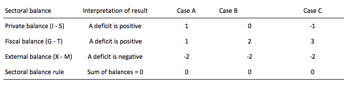
To help us answer the specific question posed, we can identify three states all involving public and external deficits:

• Case A: Fiscal Deficit (G – T) < Current Account balance (X – M) deficit.
• Case B: Fiscal Deficit (G – T) = Current Account balance (X – M) deficit.
• Case C: Fiscal Deficit (G – T) > Current Account balance (X – M) deficit.

The following Table shows these three cases expressing the balances as percentages of GDP. Case A shows the situation where the external deficit exceeds the public deficit and the private domestic sector is in deficit. In this case, there can be no overall private sector de-leveraging.

With the external balance set at a 2 per cent of GDP, as the budget moves into larger deficit, the private domestic balance approaches balance (Case B). Case B also does not permit the private sector to save overall.

Once the fiscal deficit is large enough (3 per cent of GDP) to offset the demand-draining external deficit (2 per cent of GDP) the private domestic sector can save overall (Case C).

In this situation, the fiscal deficits are supporting aggregate spending which allows income growth to be sufficient to generate savings greater than investment in the private domestic sector but have to be able to offset the demand-draining impacts of the external deficits to provide sufficient income growth for the private domestic sector to save.

For the domestic private sector (households and firms) to reduce their overall levels of debt they have to net save overall. The behavioural implications of this accounting result would manifest as reduced consumption or investment, which, in turn, would reduce overall aggregate demand.

The normal inventory-cycle view of what happens next goes like this. Output and employment are functions of aggregate spending. Firms form expectations of future aggregate demand and produce accordingly. They are uncertain about the actual demand that will be realised as the output emerges from the production process.

The first signal firms get that household consumption is falling is in the unintended build-up of inventories. That signals to firms that they were overly optimistic about the level of demand in that particular period.

Once this realisation becomes consolidated, that is, firms generally realise they have over-produced, output starts to fall. Firms lay-off workers and the loss of income starts to multiply as those workers reduce their spending elsewhere.

At that point, the economy is heading for a recession.

So the only way to avoid these spiralling employment losses would be for an exogenous intervention to occur. Given the question assumes on-going external deficits, the implication is that the exogenous intervention would come from an expanding public deficit. Clearly, if the external sector improved the expansion could come from net exports.

It is possible that at the same time that the households and firms are reducing their consumption in an attempt to lift the saving ratio, net exports boom. A net exports boom adds to aggregate demand (the spending injection via exports is greater than the spending leakage via imports).

So it is possible that the public fiscal balance could actually go towards surplus and the private domestic sector increase its saving ratio if net exports were strong enough.

The important point is that the three sectors add to demand in their own ways. Total GDP and employment are dependent on aggregate demand. Variations in aggregate demand thus cause variations in output (GDP), incomes and employment. But a variation in spending in one sector can be made up via offsetting changes in the other sectors.

The following blogs may be of further interest to you:

• Private deleveraging requires fiscal support
• Stock-flow consistent macro models
• Norway and sectoral balances
• The OECD is at it again!
• Saturday Quiz – May 22, 2010 – answers and discussion

Question 3:

The imposition of fiscal rules which aim to limit the discretionary capacity of governments to net spend bias fiscal policy towards counter-cyclical responses when private spending is weak.

The answer is False.

The non-government sector spending decisions ultimately determine the fiscal balance associated with any discretionary fiscal policy.

The fiscal balance has two conceptual components. First, the part that is associated with the chosen (discretionary) fiscal stance of the government independent of cyclical factors. So this component is chosen by the government.

Second, the cyclical component which refer to the automatic stabilisers that operate in a counter-cyclical fashion. When economic growth is strong, tax revenue improves given it is typically tied to income generation in some way. Further, most governments provide transfer payment relief to workers (unemployment benefits) and this decreases during growth.

In times of economic decline, the automatic stabilisers work in the opposite direction and push the fiscal balance towards deficit, into deficit, or into a larger deficit. These automatic movements in aggregate demand play an important counter-cyclical attenuating role. So when GDP is declining due to falling aggregate demand, the automatic stabilisers work to add demand (falling taxes and rising welfare payments).

When GDP growth is rising, the automatic stabilisers start to pull demand back as the economy adjusts (rising taxes and falling welfare payments).

The cyclical component is not insignificant and if the swings in private spending are significant then there will be significant swings in the fiscal balance.

The importance of this component is that the government cannot reliably target a particular deficit outcome with any certainty. This is why adherence to fiscal rules are fraught and normally lead to pro-cyclical fiscal policy which is usually undesirable, especially when the economy is in recession.

The fiscal outcome is thus considered to be endogenous – that is, it is determined by private spending (saving) decisions. The government can set its discretionary net spending at some target to target a particular fiscal deficit outcome but it cannot control private spending fluctuations which will ultimately determine the final actual fiscal balance.

The following blogs may be of further interest to you:

• Saturday Quiz – May 1, 2010 – answers and discussion
• Understanding central bank operations
• Building bank reserves will not expand credit
• Building bank reserves is not inflationary
• Deficit spending 101 – Part 1
• Deficit spending 101 – Part 2
• Deficit spending 101 – Part 3
• A modern monetary theory lullaby
• Saturday Quiz – April 24, 2010 – answers and discussion
• The dreaded NAIRU is still about!
• Structural deficits – the great con job!
• Structural deficits and automatic stabilisers
• Another economics department to close

That is enough for today!

(c) Copyright 2018 William Mitchell. All Rights Reserved.