The Weekend Quiz – October 27-28, 2018 – answers and discussion

Here are the answers with discussion for this Weekend’s Quiz. The information provided should help you work out why you missed a question or three! If you haven’t already done the Quiz from yesterday then have a go at it before you read the answers. I hope this helps you develop an understanding of Modern Monetary Theory (MMT) and its application to macroeconomic thinking. Comments as usual welcome, especially if I have made an error.

Question 1:

Only one of the following propositions is possible (with all balances expressed as a per cent of GDP):

• A nation can export less than the sum of imports, net factor income (such as interest and dividends) and net transfer payments (such as foreign aid) and run a government surplus of equal proportion to GDP, while the private domestic sector is spending less than they are earning.
• A nation can export less than the sum of imports, net factor income (such as interest and dividends) and net transfer payments (such as foreign aid) and run a government sector surplus of equal proportion to GDP, while the private domestic sector is spending more than they are earning.
• A nation can export less than the sum of imports, net factor income (such as interest and dividends) and net transfer payments (such as foreign aid) and run a government sector surplus that is larger, while the private domestic sector is spending less than they are earning.
• None of the above are possible as they all defy the sectoral balances accounting identity.

The correct answer is the Option (b) – “A nation can run a current account deficit accompanied by a government sector surplus of equal proportion to GDP, while the private domestic sector is spending more than they are earning”.

Note that the the current account is equal to the trade balance plus invisibles. The trade balance is exports minus imports and the invisibles are equal to the sum of net factor income (such as interest and dividends) and net transfer payments (such as foreign aid). So the question is asking about a current account deficit.

This is a question about the sectoral balances – the government fiscal balance, the external balance and the private domestic balance – that have to always add to zero because they are derived as an accounting identity from the national accounts.

To refresh your memory the balances are derived as follows. The basic income-expenditure model in macroeconomics can be viewed in (at least) two ways: (a) from the perspective of the sources of spending; and (b) from the perspective of the uses of the income produced. Bringing these two perspectives (of the same thing) together generates the sectoral balances.

From the sources perspective we write:

(1) GDP = C + I + G + (X – M)

which says that total national income (GDP) is the sum of total final consumption spending (C), total private investment (I), total government spending (G) and net exports (X – M).

Expression (1) tells us that total income in the economy per period will be exactly equal to total spending from all sources of expenditure.

We also have to acknowledge that financial balances of the sectors are impacted by net government taxes (T) which includes all tax revenue minus total transfer and interest payments (the latter are not counted independently in the expenditure Expression (1)).

Further, as noted above the trade account is only one aspect of the financial flows between the domestic economy and the external sector. we have to include net external income flows (FNI).

Adding in the net external income flows (FNI) to Expression (2) for GDP we get the familiar gross national product or gross national income measure (GNP):

(2) GNP = C + I + G + (X – M) + FNI

To render this approach into the sectoral balances form, we subtract total net taxes (T) from both sides of Expression (3) to get:

(3) GNP – T = C + I + G + (X – M) + FNI – T

Now we can collect the terms by arranging them according to the three sectoral balances:

(4) (GNP – C – T) – I = (G – T) + (X – M + FNI)

The the terms in Expression (4) are relatively easy to understand now.

The term (GNP – C – T) represents total income less the amount consumed less the amount paid to government in taxes (taking into account transfers coming the other way). In other words, it represents private domestic saving.

The left-hand side of Equation (4), (GNP – C – T) – I, thus is the overall saving of the private domestic sector, which is distinct from total household saving denoted by the term (GNP – C – T).

In other words, the left-hand side of Equation (4) is the private domestic financial balance and if it is positive then the sector is spending less than its total income and if it is negative the sector is spending more than it total income.

The term (G – T) is the government financial balance and is in deficit if government spending (G) is greater than government tax revenue minus transfers (T), and in surplus if the balance is negative.

Finally, the other right-hand side term (X – M + FNI) is the external financial balance, commonly known as the current account balance (CAD). It is in surplus if positive and deficit if negative.

In English we could say that:

The private financial balance equals the sum of the government financial balance plus the current account balance.

We can re-write Expression (6) in this way to get the sectoral balances equation:

(5) (S – I) = (G – T) + CAD

which is interpreted as meaning that government sector deficits (G – T > 0) and current account surpluses (CAD > 0) generate national income and net financial assets for the private domestic sector.

Conversely, government surpluses (G – T < 0) and current account deficits (CAD < 0) reduce national income and undermine the capacity of the private domestic sector to add financial assets.

Expression (5) can also be written as:

(6) [(S – I) – CAD] = (G – T)

where the term on the left-hand side [(S – I) – CAD] is the non-government sector financial balance and is of equal and opposite sign to the government financial balance.

This is the familiar MMT statement that a government sector deficit (surplus) is equal dollar-for-dollar to the non-government sector surplus (deficit).

The sectoral balances equation says that total private savings (S) minus private investment (I) has to equal the public deficit (spending, G minus taxes, T) plus net exports (exports (X) minus imports (M)) plus net income transfers.

All these relationships (equations) hold as a matter of accounting and not matters of opinion.

Thus, when an external deficit (X – M < 0) and public surplus (G – T < 0) coincide, there must be a private deficit. While private spending can persist for a time under these conditions using the net savings of the external sector, the private sector becomes increasingly indebted in the process.

Note we are ignoring the FNI component here – assuming it is zero.

Second, you then have to appreciate the relative sizes of these balances to answer the question correctly.

The rule is that the sectoral balances have to sum to zero. So if we write the condition above as:

(S – I) – (G – T) – (X – M) = 0

Or:

(S – I) = (G – T) + (X – M)

Assume:

(X – M) = -2 (an external deficit)

(G – T) = -2 (a fiscal surplus)

Then we would get:

(S – I) = -2 + (-2) = -4 (a private domestic deficit)

If (G – T) was -3 (a larger surplus)

Then:

(S – I) = -3 + (-2) = -5 (a larger private domestic deficit)

This tells us that even if the external sector is growing strongly and is in surplus there may still be a need for public deficits. This will occur if the private domestic sector seek to save at a proportion of GDP higher than the external surplus.

The economics of this situation might be something like this. The external surplus would be adding to overall aggregate demand (the injection from exports exceeds the drain from imports). However, if the drain from private sector spending (S > I) is greater than the external injection then the only way output and income can remain constant is if the government is in deficit.

National income adjustments would occur if the private domestic sector tried to push for higher saving overall – income would fall (because overall spending fell) and the government would be pushed into deficit whether it liked it or not via falling revenue and rising welfare payments.

The following Table represents the three options in percent of GDP terms. To aid interpretation remember that (S-I) < 0 means that the private domestic sector is spending more than they are earning; that (G-T) < 0 means that the government is running a surplus because T > G; and (X-M) < 0 means the external position is in deficit because imports are greater than exports.

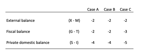
The first two possibilities we might call A and B:

A: A nation can run a current account deficit with an offsetting government sector surplus, while the private domestic sector is spending less than they are earn

B: A nation can run a current account deficit with an offsetting government sector surplus, while the private domestic sector is spending more than they are earning.

So Option A says the private domestic sector is saving overall, whereas Option B say the private domestic sector is dis-saving (and going into increasing indebtedness). These options are captured in the first two columns of the Table.

So the arithmetic example depicts an external sector deficit of 2 per cent of GDP and an offsetting fiscal surplus of 2 per cent of GDP.

You can see that the private sector balance is negative (that is, the sector is spending more than they are earning – Investment is greater than Saving – and has to be equal to 4 per cent of GDP.

Given that the only proposition that can be true is:

B: A nation can run a current account deficit with an offsetting government sector surplus, while the private domestic sector is spending more than they are earning.

Column 2 in the Table captures Option C:

C: A nation can run a current account deficit with a government sector surplus that is larger, while the private domestic sector is spending less than they are earning.

So the current account deficit is equal to 2 per cent of GDP while the surplus is now larger at 3 per cent of GDP. You can see that the private domestic deficit rises to 5 per cent of GDP to satisfy the accounting rule that the balances sum to zero.

The final option available is:

D: None of the above are possible as they all defy the sectoral balances accounting identity.

It cannot be true because as the Table data shows the rule that the sectoral balances add to zero because they are an accounting identity is satisfied in both cases.

So if the G is spending less than it is “earning” and the external sector is adding less income (X) than it is absorbing spending (M), then the other spending components must be greater than total income.

You may wish to read the following blogs for more information:

• Back to basics – aggregate demand drives output
• Stock-flow consistent macro models
• Norway and sectoral balances
• The OECD is at it again!
• Barnaby, better to walk before we run
• Saturday Quiz – June 19, 2010 – answers and discussion

Question 2:

For workers to regain a larger share of national income, nominal wages have to grow faster than inflation – that is, the real wage has to rise.

The answer is False.

The wage share in nominal GDP is expressed as the total wage bill as a percentage of nominal GDP. Economists differentiate between nominal GDP ($GDP), which is total output produced at market prices and real GDP (GDP), which is the actual physical equivalent of the nominal GDP. We will come back to that distinction soon.

To compute the wage share we need to consider total labour costs in production and the flow of production ($GDP) each period.

Employment (L) is a stock and is measured in persons (averaged over some period like a month or a quarter or a year.

The wage bill is a flow and is the product of total employment (L) and the average wage (w) prevailing at any point in time. Stocks (L) become flows if it is multiplied by a flow variable (W). So the wage bill is the total labour costs in production per period.

So the wage bill = W.L

The wage share is just the total labour costs expressed as a proportion of $GDP – (W.L)/$GDP in nominal terms, usually expressed as a percentage. We can actually break this down further.

Labour productivity (LP) is the units of real GDP per person employed per period. Using the symbols already defined this can be written as:

LP = GDP/L

so it tells us what real output (GDP) each labour unit that is added to production produces on average.

We can also define another term that is regularly used in the media – the real wage – which is the purchasing power equivalent on the nominal wage that workers get paid each period. To compute the real wage we need to consider two variables: (a) the nominal wage (W) and the aggregate price level (P).

The nominal wage (W) – that is paid by employers to workers is determined in the labour market – by the contract of employment between the worker and the employer. The price level (P) is determined in the goods market – by the interaction of total supply of output and aggregate demand for that output although there are complex models of firm price setting that use cost-plus mark-up formulas with demand just determining volume sold. We shouldn’t get into those debates here.

The inflation rate is just the continuous growth in the price level (P). A once-off adjustment in the price level is not considered by economists to constitute inflation.

So the real wage (w) tells us what volume of real goods and services the nominal wage (W) will be able to command and is obviously influenced by the level of W and the price level. For a given W, the lower is P the greater the purchasing power of the nominal wage and so the higher is the real wage (w).

We write the real wage (w) as W/P. So if W = 10 and P = 1, then the real wage (w) = 10 meaning that the current wage will buy 10 units of real output. If P rose to 2 then w = 5, meaning the real wage was now cut by one-half.

So the proposition in the question – that nominal wages grow faster than inflation – tells us that the real wage is rising.

Nominal GDP ($GDP) can be written as P.GDP, where the P values the real physical output.

Now if you put of these concepts together you get an interesting framework. To help you follow the logic here are the terms developed and be careful not to confuse $GDP (nominal) with GDP (real):

• Wage share = (W.L)/$GDP
• Nominal GDP: $GDP = P.GDP
• Labour productivity: LP = GDP/L
• Real wage: w = W/P

By substituting the expression for Nominal GDP into the wage share measure we get:

Wage share = (W.L)/P.GDP

In this area of economics, we often look for alternative way to write this expression – it maintains the equivalence (that is, obeys all the rules of algebra) but presents the expression (in this case the wage share) in a different “view”.

So we can write as an equivalent:

Wage share – (W/P).(L/GDP)

Now if you note that (L/GDP) is the inverse (reciprocal) of the labour productivity term (GDP/L). We can use another rule of algebra (reversing the invert and multiply rule) to rewrite this expression again in a more interpretable fashion.

So an equivalent but more convenient measure of the wage share is:

Wage share = (W/P)/(GDP/L) – that is, the real wage (W/P) divided by labour productivity (GDP/L).

I won’t show this but I could also express this in growth terms such that if the growth in the real wage equals labour productivity growth the wage share is constant. The algebra is simple but we have done enough of that already.

That journey might have seemed difficult to non-economists (or those not well-versed in algebra) but it produces a very easy to understand formula for the wage share.

Two other points to note. The wage share is also equivalent to the real unit labour cost (RULC) measures that Treasuries and central banks use to describe trends in costs within the economy. Please read my blog – Saturday Quiz – May 15, 2010 – answers and discussion – for more discussion on this point.

Now it becomes obvious that if the nominal wage (W) grows faster than the price level (P) then the real wage is growing. But that doesn’t automatically lead to a growing wage share. So the blanket proposition stated in the question is false.

If the real wage is growing at the same rate as labour productivity, then both terms in the wage share ratio are equal and so the wage share is constant.

If the real wage is growing but labour productivity is growing faster, then the wage share will fall.

Only if the real wage is growing faster than labour productivity , will the wage share rise.

The wage share was constant for a long time during the Post Second World period and this constancy was so marked that Kaldor (the Cambridge economist) termed it one of the great “stylised” facts. So real wages grew in line with productivity growth which was the source of increasing living standards for workers.

The productivity growth provided the “room” in the distribution system for workers to enjoy a greater command over real production and thus higher living standards without threatening inflation.

Since the mid-1980s, the neo-liberal assault on workers’ rights (trade union attacks; deregulation; privatisation; persistently high unemployment) has seen this nexus between real wages and labour productivity growth broken. So while real wages have been stagnant or growing modestly, this growth has been dwarfed by labour productivity growth.

Question 3:

Economists use rules of thumb to make estimates of the future direction of key aggregates based upon assumptions about the movement in related aggregates. Say, we form the view that over the next year: (a) the average working week will be constant in hours; (b) real GDP growth rate will be 3 per cent; (c) output per unit of labour input (persons) grows at 1.5 per cent; and (d) the labour force maintains a growth rate of 1.5 per cent per annum. We would project that the:

(a) The unemployment rate will rise in the coming year by 1.5 per cent.

(b) The unemployment rate will fall in the coming year by 1.5 per cent.

(c) The unemployment rate will be unchanged.

The answer is Option (c) – the unemployment rate will be unchanged.

The assumptions made about the aggregates over the next 12 months were:

• Real GDP growth growth rate of 3 per cent annum.
• Labour productivity growth (that is, growth in real output per person employed) growing at 1.5 per cent per annum. So as this grows less employment in required per unit of output.
• The labour force is growing by 1.5 per cent per annum. Growth in the labour force adds to the employment that has to be generated for unemployment to stay constant (or fall).
• The average working week is constant in hours. So firms are not making hours adjustments up or down with their existing workforce. Hours adjustments alter the relationship between real GDP growth and persons employed.

The real GDP growth rate doesn’t relate to the labour market in any direct way. The late Arthur Okun is famous (among other things) for estimating the relationship that links the percentage deviation in real GDP growth from potential to the percentage change in the unemployment rate – the so-called Okun’s Law.

The algebra underlying this law can be manipulated to estimate the evolution of the unemployment rate based on real output forecasts.

From Okun, we can relate the major output and labour-force aggregates to form expectations about changes in the aggregate unemployment rate based on output growth rates. A series of accounting identities underpins Okun’s Law and helps us, in part, to understand why unemployment rates have risen.

Take the following output accounting statement:

(1) Y = LP*(1-UR)LH

where Y is real GDP, LP is labour productivity in persons (that is, real output per unit of labour), H is the average number of hours worked per period, UR is the aggregate unemployment rate, and L is the labour-force. So (1-UR) is the employment rate, by definition.

Equation (1) just tells us the obvious – that total output produced in a period is equal to total labour input [(1-UR)LH] times the amount of output each unit of labour input produces (LP).

Using some simple calculus you can convert Equation (1) into an approximate dynamic equation expressing percentage growth rates, which in turn, provides a simple benchmark to estimate, for given labour-force and labour productivity growth rates, the increase in output required to achieve a desired unemployment rate.

Accordingly, with small letters indicating percentage growth rates and assuming that the average number of hours worked per period is more or less constant, we get:

(2) y = lp + (1 – ur) + lf

Re-arranging Equation (2) to express it in a way that allows us to achieve our aim (re-arranging just means taking and adding things to both sides of the equation):

(3) ur = 1 + lp + lf – y

Equation (3) provides the approximate rule of thumb – if the unemployment rate is to remain constant, the rate of real output growth must equal the rate of growth in the labour-force plus the growth rate in labour productivity.

It is an approximate relationship because cyclical movements in labour productivity (changes in hoarding) and the labour-force participation rates can modify the relationships in the short-run. But it provides reasonable estimates of what happens when real output changes.

The sum of labour force and productivity growth rates is referred to as the required real GDP growth rate – required to keep the unemployment rate constant.

Remember that labour productivity growth (real GDP per person employed) reduces the need for labour for a given real GDP growth rate while labour force growth adds workers that have to be accommodated for by the real GDP growth (for a given productivity growth rate).

So in the example, the required real GDP growth rate is 3 per cent per annum and so the actual real GDP growth is also equal to this required real GDP growth rate. In other words, the unemployment rate will remain unchanged.

Unemployment would still be rising but the rate of unemployment will be constant.

The following blog may be of further interest to you:

• What do the IMF growth projections mean?

That is enough for today!

(c) Copyright 2018 William Mitchell. All Rights Reserved.