It’s Wednesday and I just finished a ‘Conversation’ with the Economics Society of Australia, where I talked about Modern Monetary Theory (MMT) and its application to current policy issues. Some of the questions were excellent and challenging to answer, which is the best way. You can view an edited version of the discussion below and…
IS-LM Framework – Part 4
I am now using Friday’s blog space to provide draft versions of the Modern Monetary Theory textbook that I am writing with my colleague and friend Randy Wray. We expect to complete the text during 2013 (to be ready in draft form for second semester teaching). Comments are always welcome. Remember this is a textbook aimed at undergraduate students and so the writing will be different from my usual blog free-for-all. Note also that the text I post is just the work I am doing by way of the first draft so the material posted will not represent the complete text. Further it will change once the two of us have edited it.
Previous Parts to this Chapter:
Chapter 16 – The IS-LM Framework
[PREVIOUS MATERIAL HERE IN PARTS 1, 2 and 3]
16.5 Policy analysis in IS-LM
The IS-LM framework is used within the mainstream approach to analyse the impact of fiscal and monetary policy changes on output (income) and interest rates, and by implication, employment.
Monetary policy is represented by the assumed capacity of the central bank to alter the money supply. Inherent in this appraoch is the view that central banks manipulate base money (reserves) which are then transmitted into a broader money supply via the money multiplier mechanisms.
In Chapter 9, we demonstrated how this view of central bank operations is not a valid representation of the real world and that, in fact, the central bank has little control over the money supply and conducts monetary policy principally via its capacity to set the short-term interest rate. However, for the purposes of this Chapter, to ensure we render the IS-LM approach faithfully, we assume the money supply is exogenous and under the control of the central bank.
Monetary policy changes are thus represented in the IS-LM framework by shifts in the LM curve.
Figure 16.2 showed that if the central bank increases the money supply, the interest rate falls at the current national income level. This is because at the existing interest rate, there is an excess supply of money and the interest rate has to fall to stimulate an increased demand for money.
The interest rate continues to fall until the demand for money is again equal to the increased money supply and money market equilibrium is restored.
In terms of the LM curve, this means that at higher levels of money supply, equilibrium interest rates will be lower at each income level which translates into a shift outwards in the LM curve. The opposite occurs when the money supply falls.
| The LM curve shifts to the right when the money supply rises and shifts to the left when the money supply contracts. |
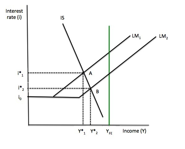
Figure 16.7 shows the impacts of expansionary monetary policy. At some existing monetary policy stance captured by LM1 the equilibrium combination of the interest rate and national income is i*1, Y*1. Point A shows the equilibrium position where LM1 cuts the IS curve.
The central bank decides that the output gap (measured by the difference between the full employment national income level, YFE and the current national income level, Y*1) is intolerable (given the implied mass unemployment that would be associated with such a deficiency in output) and they increase the money supply.
The LM curve shifts to LM2, which drives down interest rates (to stimulate a higher demand for money). The new equilibrium is at Point B, with the equilibrium combination of the interest rate and national income at i*2, Y*2.
The rising income results from the positive impact on investment of the lower interest rates (represented by the movement along the IS curve from A to B). The more sensitive is investment spending to interest rate changes the more expansionary the monetary policy change will be.
Note, that in this case, monetary policy would not be able to achieve full employment because the economy would encounter a liquidity trap (at i0) before full employment was restored.
A contractionary monetary policy could be represented in Figure 16.7 by a shift in the LM curve from LM2 to LM1. This would drive interest rates up and national income down.
The falling income results from the negative impact on investment of the higher interest rates (represented by the movement along the IS curve from B to A). The more sensitive is investment spending to interest rate changes the more contractinoary the monetary policy change will be.
Figure 16.7 Expansionary Monetary Policy

|
Expansionary monetary policy drives the interest rate down and national income up. Contractionary monetary policy drives the interest rate up and national income down.
The extent of the expansion or contraction depends on the slope of the IS curve. The steeper the IS curve the less effective are monetary policy changes with respect to income changes. |
Fiscal policy changes could be implemented by discretionary changes in government spending or the tax rate. We have learned that a rise in government spending shifts the IS curve to the right because for a given interest rate, the equilibrium level of national income rises when autonomous spending rises.
Similarly, a fall in government spending shifts the IS curve to the left because for a given interest rate, the equilibrium level of national income falls when autonomous spending falls.
The magnitude of the shift up or down in the IS resulting from a rise (fall) in autonomous spending is determined by the magnitude of the change in autonomous spending and the size of the expenditure multiplier.
For a given change in autonomous spending, the shift in the IS curve will be larger, the larger is the value of the expenditure multiplier.
| The IS curve shifts to the right when government spending rises and shifts to the left when the government spending falls. |
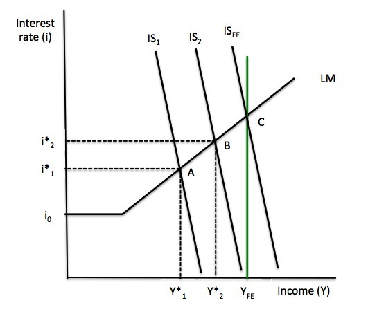
Figure 16.8 depicts an expansionary fiscal policy change (increase in government spending). At some existing fiscal policy stance captured by IS1 the equilibrium combination of the interest rate and national income is i*1, Y*1. Point A shows the equilibrium position where IS1 cuts the LM curve.
The treasury decides that the output gap (measured by the difference between the full employment national income level, YFE and the current national income level, Y*1) is intolerable (given the implied mass unemployment that would be associated with such a deficiency in output) and they increase government spending in order to stimulate aggregate demand.
The IS curve shifts to IS2 which creates a new equilibrium at Point B, with the equilibrium combination of the interest rate and national income at i*2, Y*2.
You will note that both the interest rate and national income are higher. The rising national income arises because at higher levels of aggregate demand, firms produce more output (and hire more workers).
How do we explain the higher interest rates? Within the IS-LM framework, the rising national income that follows the increased aggregate demand, increases the transactions demand for money. With the money supply fixed, the rising demand for money creates an excess demand for money at the original equilibrium interest rate (i*1) and rising interest rates motivate people to hold less cash. This is because the opportunity cost of holding wealth in the form of cash rises when interest rates rise.
You will note that if the interest rates had not have increased, the expansion in income would have been greater than the shift from Y*1 to Y*2.
Figure 16.8 Expansionary Fiscal Policy

The final change in aggregate demand is thus less than the initial ΔG. How do we explain this?
The rising interest rates impact negatively on private investment which offsets some of the increase in government spending. In the policy debates this impact is referred to as financial crowding out. The rising interest rates that follow the increase in government spending, crowd out other interest sensitive components of aggregate demand (in this case, private investment).
Note that fiscal policy could achieve full employment (at Point C) if the government kept increasing government spending such that the IS curve shifted to ISFE.
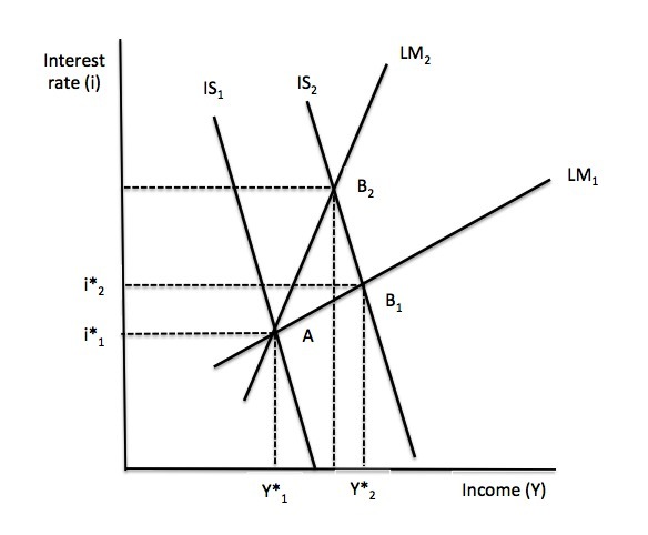
The extent of the financial crowding out depends on the slope of the LM curve. The steeper is the LM curve the less expansionary will fiscal policy be and the larger is the crowding out effects.
This is demonstrated in Figure 16.9. From an initial equilibrium at Point A, a fiscal stimulus (shifting IS curve to IS2) would increase national income to Y*2 and interest rate would rise to i*2 with the flatter LM curve (LM1) at the new equilibrium point, B1.
With a steeper LM curve (LM2), for the same fiscal stimulus (shifting IS curve to IS2), the new equilibrium point, B2 clearly involves a lower equilibrium income outcome and a higher equilibrium interest rate than occurred at Point B1.
The extent of the financial crowding out is higher with LM2 than LM1.
What explains this difference? The LM curve is steeper the more sensitive the demand for money (transactions and precautionary motives) is to national income changes and the less sensitive the speculative demand for money is to changes in interest rates.
Thus, small changes in national income lead to large changes in excess money demand at a given money supply level and the rise in interest rates to restore money market equilibrium, other things equal, has to be larger as a consequence. Additionally, for a given excess demand for money, the interest rate increase that is required to restore money market equilibrium is larger.
A extreme position is complete financial crowding out and this would occur if the LM curve was vertical. In this situation a given rise in government spending, for example, would be exactly offset by a decline in investment as the interest rate rose.
In that situation, fiscal policy would be totally ineffective.
We should note that financial crowding out is not confined to fiscal policy changes exclusively. Any of the autonomous spending components, which can shift the IS curve and increase national income, trigger the money market mechanisms that see interest rates rise and interest-sensitive components of aggregate demand stifled.
Figure 16.9 Fiscal policy and financial crowding out

Note that the other extreme position would be a horizontal LM curve at some given interest rate. In this case there would be no financial crowding out and the fiscal stimulus to aggregate demand would be fully translated into changes in national income.
We will return to this extreme position when we discuss endogenous money theories later in the Chapter.
|
An expansionary fiscal policy change increases national income and interest rates.
The rise in national income is less than the change in government spending because the higher interest rates crowd out private investment. The extent of the financial crowding out depends on the slope of the LM curve. The steeper is the LM curve the less expansionary will fiscal policy be and the larger is the crowding out effects. There is complete crowding out when the LM curve is vertical and zero crowding out when the LM curve is horizontal. |
16.6 Introducing the price level
Our derivation of the IS-LM framework initially assumed that the price level was fixed and all changes in output were real. This is consistent with the simple income-expenditure model developed in Chapter 12 where the focus was on the manner in which output and employment responds to changes in aggregate demand.
We assumed that firms were willing to supply whatever was demanded up to full capacity without changing their prices.
In this vein, we also treated the nominal and real interest rate has being interchangeable.
In this section we consider how changes in the price level impact on output and interest rates.
[TO BE CONTINUED IN PART 5]
Conclusion
PART 5 next week – Introducing the Price Level to the Analysis – PIGOU AND KEYNES EFFECTS AND CRITIQUE OF FRAMEWORK.
Saturday Quiz
The Saturday Quiz will be back again tomorrow. It will be of an appropriate order of difficulty (-:
That is enough for today!
(c) Copyright 2013 Bill Mitchell. All Rights Reserved.
“The rising interest rates impact negatively on private investment which offsets some of the increase in government spending.”
Not if the government spending increased the returns from private investment more than the increase in the interest rate. Eg new infrastructure spending etc..
Steve,
All the gaping holes you or I could point out in the IS-LM framework Bill has pointed out numerous times before. He is including it in his textbook because it is widely used in the current debate and he believes it is important for students to understand it. I am sure he will have a section with critique and analysis.
Hi,
here are my comments:
“In terms of the LM curve, this means that at higher levels of money supply, equilibrium interest rates will be lower at each income level which translates into a shift outwards in the LM curve. The opposite occurs when the money supply falls.”
This could be described in more proper language which reflects that money supply is being pushed around as a policy variable. The last sentence makes money supply a player on its own, maybe better would be: “The opposite occurs when the money supply is decreased (by the central bank).”
“The central bank decides that the output gap (measured by the difference between the full employment national income level, YFE and the current national income level, Y*1) is intolerable (given the implied mass unemployment that would be associated with such a deficiency in output) and they increase the money supply.”
A deficiency in output does not have to be “mass unemployment”, it could start a stage below with “some unemployment”. IS/LM is (normally) not shown to apply only in a depression.
“The IS curve shifts to the right when government spending rises and shifts to the left when the government spending falls.”
A little below you mentioned changes in the tax rate. These should be mentioned in the above section again. Also, it might be interesting to add a quick discussion of policy effectiveness (tax cuts vs fiscal stimulus – maybe in an additional box?).
best,
Dirk