It’s Wednesday and I just finished a ‘Conversation’ with the Economics Society of Australia, where I talked about Modern Monetary Theory (MMT) and its application to current policy issues. Some of the questions were excellent and challenging to answer, which is the best way. You can view an edited version of the discussion below and…
The IS-LM Framework – Part 3
I am now using Friday’s blog space to provide draft versions of the Modern Monetary Theory textbook that I am writing with my colleague and friend Randy Wray. We expect to complete the text during 2013 (to be ready in draft form for second semester teaching). Comments are always welcome. Remember this is a textbook aimed at undergraduate students and so the writing will be different from my usual blog free-for-all. Note also that the text I post is just the work I am doing by way of the first draft so the material posted will not represent the complete text. Further it will change once the two of us have edited it.
Previous Parts to this Chapter:
Chapter 16 – The IS-LM Framework
[PREVIOUS MATERIAL HERE IN PARTS 1 and 2]
We thus have two combinations of interest rates and income levels which are consistent with product market equilibrium. Clearly we could trace out the impact of many interest rate changes and thus many equilibrium combinations of interest rates and income.
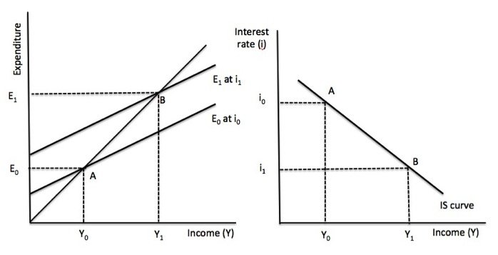
The IS curve is the line that joins all the equilibrium combinations of interest rates and national income. Figure 16.5 shows this derivation.
Figure 16.5 The derivation of the IS curve

Point A is one product equilibrium where the interest rate is i0 and total expenditure is E0 generating total national income of Y0.
In the right-hand panel where the interest rate is on the vertical axis and national income is on the horizontal axis, point A shows the combination of the interest rate and income which produce the product market equilibrium shown in the left-hand pane.
If interest rates fell to i1, total expenditure rises to E1 as a result of the higher investment expenditure, which leads to a rise in national income via the expenditure multiplier. Point B shows the new product market equilibrium at (i1, Y1).
We could examine the impact of any number of interest rate changes on product market equilibrium in the left panel and subsequently map these points into the right panel. The result would be the IS curve.
The IS curve therefore is a series of points corresponding to equilibrium combinations of national income and interest rates in the product market.
It is clear that in the IS-LM framework, the money market impacts on the product market through the impact of interest rate changes on investment. The change in income results from the initial response of investment to an interest rate change then being multiplied through the expenditure system via induced consumption and leakages to taxation and imports.
In other words, the total change in income that follows a change in the interest rate depends on the values of the expenditure multiplier and the sensitivity of investment to interest rate changes.
What factors will shift the IS curve? First, any increase (decrease) in autonomous spending shifts IS up (down) because for a given interest rate, the equilibrium level of national income rises (falls) when autonomous spending rises (falls).
The magnitude of the shift up or down in the IS resulting from a rise (fall) in autonomous spending is determined by the magnitude of the change in autonomous spending and the size of the expenditure multiplier.
For a given change in autonomous spending, the shift in the IS curve will be larger the larger is the value of the expenditure multiplier.
The slope of the IS curve represents this overall sensitivity of national income to interest rate changes. The larger is the expenditure multiplier and the larger is the sensitivity of investment to interest rate changes the flatter the IS curve.
This is because for a given change in interest rates, the initial response of investment spending will be larger the more responsive it is to the cost of capital, other things being equal.
In turn, a given change in investment will generate a larger (smaller) change in national income the larger (smaller) is the value of the expenditure multiplier.
If current period investment is very unresponsive to a change in the current interest rate then the IS curve will be very steep. It is argued by economists who consider time to be an important consideration in economic analysis that investment spending plans are based on expectations of future revenue streams that were formed in past periods.
The current period’s flow of investment spending reflects these past decisions. The time it takes to evaluate different projects, design the appropriate necessary capital equipment, source funding and then implement the capital infrastructure suggests that current investment spending will be relatively insensitive to current changes in interest rates.
We discuss this topic more in Chapter 22.
It should be clear from this discussion that changes in the tax rate (t), which impact on the value of the expenditure multiplier will also impact on the slope of the IS curve. For example, a rise in the tax rate will cause the IS curve to become steeper because it reduces the value of the expenditure multiplier – a larger leakage from the expenditure system.
Similarly, a rising saving propensity or propensity to import, which mean that there are larger leakages from the expenditure system each time income changes, will lead to a steeper IS curve.
16.4 General Equilibrium in the IS-LM framework
The intention of the IS-LM framework is to bring the product market and money market outcomes into a single diagram so that we can simultaneously determine the equilibrium value of national income and the interest rate. In doing so, it recognises the interdependency between these markets, a point that Keynes demonstrated clearly.
What happens in one market impacts on the other market, which then leads to feedback loops and new equilibrium outcomes in each.
The IS-LM framework thus conceives of a general equilibrium defined as the interest rate and income level that generates simultaneous equilibrium in the both the product and money markets.
In a graphical form, this equilibrium position corresponds to the intersection of the IS and LM curves. In the Advanced Material Box we derive the algebra corresponding to this general equilibrium.
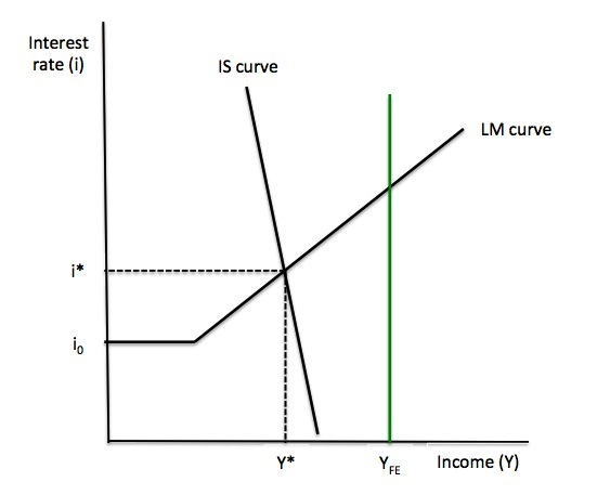
Figure 16.6 shows the IS-LM solution for equilibrium income and interest rates, Y*, i*. Two things are worth noting. The vertical green line at YFE, denotes a full employment national output level. In other words, at this output level all available labour and capital are being productively deployed.
The IS-LM joint equilibrium thus can occur at levels of income which are below full employment in the labour market. This is consistent with Keynes’ insight that the capitalist monetary system has a tendency to reach under-full employment steady states which need to be shocked by policy interventions.
At Y* and i*, business firms are selling as much as they expected to sell and have no incentive to expand production and employment. The desire for liquidity by firms and households are also being full met by the available supply of money.
This under-full employment equilibrium can be reached at interest rates above the minimum rate, where the economy enters a liquidity trap.
Figure 16.6 General IS-LM Equilibrium

[THE FOLLOWING ADVANCED MATERIAL MAY BE IN A BOX WITHIN THE CHAPTER TEXT OR PRESENTED AS A SEPARATE APPENDIX AT THE END OF THE CHAPTER]
|
Advanced material: The IS-LM algebra
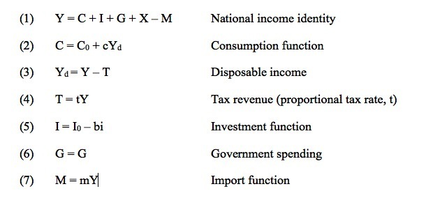
The formal IS-LM model for a simplified open economy begins with the following relationships. Product Market Product Market Equilibrium The product market equilibrium can be solved as a relationship between GDP (Y) and the interest rate (i) given the autonomous spending aggregates and the value of the multiplier. Substituting Equations (2) to (7) into (1) we get: (10) Y = C0 + cY – ctY + I0 – bi + G + X – mY Rearranging gives the equation for the IS curve: (11) Y = α(A- bi) where α = 1/(1 – c(1 – t) + m), the expenditure multiplier and A is the autonomous spending component, C0 + I0 + G + X. The slope of the IS curve is given by αb, so the larger the multiplier (α) and the sensitivity of investment to interest rates (b), the flatter will be the slope because the response of national income to a given interest rate will be larger. Money Market Equilibrium The money market equilibrium is given by the equality of money supply and money demand. (12) Ms = kY – hi Which produces the LM curve where Y is a function of i: (13) Y = (1/k)Ms + (h/k)i The slope of the LM curve is given by (h/k), so the larger the sensitivity of the demand for money to interest rates (h) and the smaller the sensitivity to income (k), the flatter will be the slope because for a small change in interest rates, a much larger change in national income will be required to maintain the equality between the demand for money and the given money supply. Equation (13) can also be written with i as a function of Y: (14) i = (k/h)Y – (1/h)Ms General Equilibrium A state of general equilibrium in this context is defined as the interest rate and income level that generates simultaneous equilibrium in the both the product and money markets. This equilibrium position corresponds to the intersection of the IS and LM curves. To solve for the equilibrium level of national income we can substitute Equation (14) into the IS curve equation (11) to give: (15) Y = α[A- (b/h)(kY – Ms)] Solving for equilibrium Y gives: Equation (16) indicates that equilibrium income is determined by autonomous spending (A), which includes the fiscal policy parameter (G) and the money supply (Ms). We use the solution in Equation (16) to solve for the equilibrium interest rate: (17) Equation (17) tells us that the equilibrium interest rate is determined by autonomous spending (A) and the money supply (Ms). Some economists use Equation (15) to define a fiscal policy multiplier, which indicates the change in national income for a given change in government spending, if the money supply is held constant. The fiscal policy multiplier is given by the coefficient on autonomous spending A in Equation (15). You will note that this is different to the expenditure multiplier, α because it takes into account the interest rate impacts of rising income on investment spending that emanate from the shifts in the demand for money in the money market. The simple expenditure multiplier is derived on the assumption that interest rates do not change when national income rises. Similarly, a monetary policy multiplier can be derived, which shows the increase in national income for a given change in the money supply, if government spending and tax rates are held constant. This is given by the coefficient on Ms in Equation (15). Note though that this assumes that monetary policy is conducted through the central bank exercising its assumed control over the money supply. This is one of the flaws of the IS-LM framework when applied to the real world – the central bank does not have control over the money supply and the assumed money multiplier does not exist in any form other than as an ex post, non-causal accounting statement. |
[TO BE CONTINUED IN PART 3]
Conclusion
PART 4 next week – Complete Chapter POLICY ANALYSIS IN THE CONTEXT OF THE CURRENT CRISIS (HOW THE IS-LM IS BEING USED BY SOME TO ANALYSE THE CRISIS), PIGOU AND KEYNES EFFECTS AND CRITIQUE OF FRAMEWORK.
Saturday Quiz
The Saturday Quiz will be back again tomorrow. It will be of an appropriate order of difficulty (-:
That is enough for today!
(c) Copyright 2013 Bill Mitchell. All Rights Reserved.


Hi,
I like the green full employment line. Another possibility would be to draw the LM curve vertical, but then you would have to talk about “crowding out”, which is nonsense. Your solution is superior.
“We thus have two combinations of interest rates and income levels which are consistent with product market equilibrium.”
There are actually two equilibrium conditions which are fulfilled simultaneously: I=S and income=expenditure. This might be confusing for students because some books use one condition, some the other.
There is an alternative way to show the derivation of IS and LM curve which is a little bit more informative, I think. You draw a 4 quadrant schedule, with the IS curve in the NE. On the axis you have i (N), Y (E), I (W) and S (S). The investment function goes into the NW, S=I into SW and the savings function into SE. For the LM diagramm, you keep i (N) and Y (E) but then add Ls (W) and Lt (S). In the NW you draw the speculative demand, in the SE the transaction demand for money. In the SW you draw a line so that M=Ls+Lt. This will help you to explain the liquidity trap.
(11) Y = α(A- bi)
where α = 1/(1 – c(1 – t) + m), the expenditure multiplier and A is the autonomous spending component, C0 + I0 – bi + G + X.
I’m not sure here. Is autonomous spending A=C0 + I0 – bi + G + X ? or just A=C0 + I0 + G + X and we substract bi out of it in eq 11? If not is substracted twice and makes no much sense.
Dear juanbeard (at 2013/08/10 at 6:01)
You are correct – it was a cut-and-paste error. Thanks for the scrutiny.
best wishes
bill