Friday lay day

Its Friday and my declared lay day for blogging. I am currently working on some research analysing the shift in patterns of regional unemployment in Europe as a result of the GFC and the policy austerity that followed (it is an invited paper from one of the leading regional science journals). That is my most pressing deadline. The patterns that we are picking up are interesting already and will be analysed in more formal terms using spatial econometric tools. I will report more fully when the paper is finished around the end of the month. I am also working on the completion of our Modern Monetary Theory (MMT) textbook, and a book on the evolution of MMT (due later this year). Bit busy.

Here is a snapshot of some of the preliminary spatial analysis – descriptive patterns, maps and tests for spatial spill-overs (dependencies). I am doing this work with one of my colleagues at CofFEE Michael Flanagan.

The data combines the NUTS-2 and NUTS-3 regional data collection published by Eurostat. The problem in this type of study is in developing a consistent dataset. For example, large areas are missing 2001 data, namely Turkey, Denmark, most of Finland.

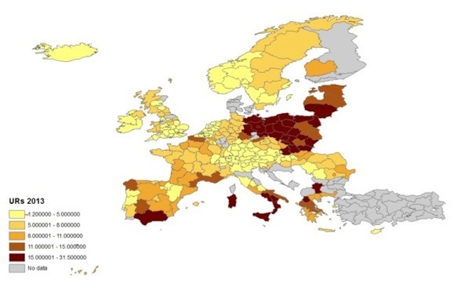
Figures 1 to 3 plot the official unemployment at the NUTS-2 level for Europe in 2001, 2007 and 2013, respectively. They thus provide a visual snapshot of the changes in the early years of euro adoption leading up to the crisis and then the post crisis period after the implementation of policy austerity.

In Figure 1 (ignore the legend title – the data is for 2001), high unemployment rates (above 15 per cent) are concentrated in the Andalucia and Murcia regions of Spain in the south, the Italian regions of Puglia, Basilicata, and Calabria and Sardegna, the northern areas of Greece, and areas of the former East Germany, parts of Poland and Slovakia and all of Latvia.

Regions with persistent unemployment rates of between 11 and 15 per cent include the Extramadura (South Central) and Galicia (North West) regions, the Puglia region in South East Italy, Southern and Northern France, Central Greece, and some regions in Poland and Estonia.

Figure 1 Official unemployment rates, Europe, 2001

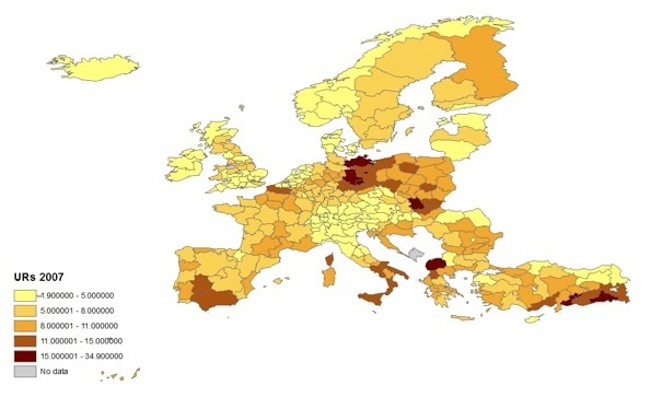
The picture had changed significantly by 2007 (see Figure 2). While economic growth was not robust it was sufficient to generate employment growth that was faster than the growth in the labour force, which meant that unemployment rates fell over the period 2001-2007.

Germany was slowly absorbing the East German economy and unemployment fell. This was partly the result of the introduction of so-called Mini-jobs under the Hartz reform agenda. But the persistently high unemployment in Southern Spain and Italy moderated (albeit remained high).

But this period was characterised by growing imbalances in trade between the south and the north of Europe and the housing booms in Ireland and Spain that drove employment growth in the construction and related industry sectors.

Further, the Baltic States were recovering after the breakdown of the Soviet system and there economies were aided by housing booms.

Figure 2 Official unemployment rates, Europe, 2007

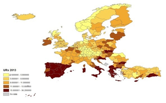
The growth came to a sudden halt with the onset of the GFC, the ensuing housing market collapse, and the subsequent imposition of fiscal austerity under the Stability and Growth Pact (SGP) saw the picture change dramatically.

Figure 3 shows the damage that had been created in terms of unemployment rates by 2013.
Relatively high unemployment rates manifest in Ireland (which had previously enjoyed very low unemployment), all of Spain and most of Portugal, all of Southern Italy, all of Greece, parts of Hungary and Slovakia.

The darkening of many other parts of the European map indicates that the level of unemployment rose more or less uniformly throughout Europe, with the main exceptions being most of Germany, Switzerland, and Norway.

Figure 3 Official unemployment rates, Europe, 2013

In order to understand the patterning of economic phenomena in large and detailed maps, such as the preceding figures, we need a way of capturing the properties of the data in a simple summary.

Exploratory Spatial Data Analysis (ESDA) is a set of techniques aimed at visualising the spatial distribution of data, identifying ‘atypical localisation’, detecting patterns of spatial association, that is clusters or hot spots and cold spots, and suggesting the presence of different spatial regimes, where data provide evidence of heterogeneity.

Measures of spatial dependence or spatial autocorrelation are a way of evaluating the amount of clustering or randomness in the data. Unlike standard measures of concentration these measures impose an explicit geographic structure, which makes them capable of summarising clustering observed via visual inspection of a map and also capable of testing whether these clusters are significantly non-random.

In order to determine if the values of unemployment in our maps deviate from one which would exist if they were randomly assigned, requires an index of comparison.

Global measures of spatial autocorrelation are such an index, providing evidence of the presence or absence of a stable pattern of dependence across our whole dataset.

NOTE: the paper will develop the tests for these measures – the results show that there is significant positive spatial autocorrelation in European unemployment rates. That means that it is much more likely that regions with high (low) unemployment have neighbours with high (low) unemployment than if the distribution of unemployment were purely random.

The pattern of European unemployment may thus be characterised by spatial segregation – regions with high unemployment rates are likely to be located nearby. Thus we can conclude that the distribution of unemployment is not random and this clustering represents a statistically significant relationship between neighbouring regions.

While our dataset reveals a globally significant trend towards clustering, global measures of spatial autocorrelation offer only an ‘average’ and can hide interesting micro-concentrations.

To overcome this limitation, local measures of spatial association (LISAs) have been developed. These indicate if one or more confined areas exhibit substantial deviation from spatial randomness.

The LISAs we use aim to identify so-called ‘hot and/or cold spots’ and to check for heterogeneity in the dataset. We use a statistic called the Getis and Ord G_i-statistic which can detect local ‘pockets’ of dependence that may not show up when using global statistics, for example they isolate micro-concentrations in the data which are otherwise swamped by data’s overall randomness.

This allows us to identify hot spots (high-high regional associations) and cold spots (low-low associations). These are statistically significant relationships between (typically) adjoining regions (or closeby neighours) where a rise in unemployment in one leads to a rise in another and vice versa.

The paper explores the behavioural factors which underlies these associations and when you see the following maps you will easily be able to appreciate that the hot spots emerged where the austerity was the harshest, the housing collapse was the greatest and the dominant industry structure most susceptible to cyclical shifts.

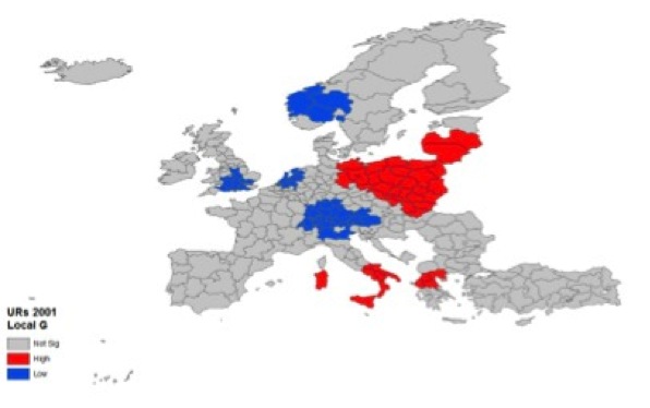
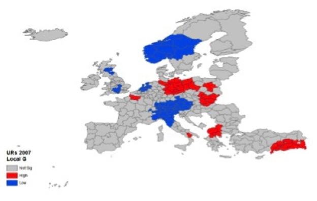
The blue coloured regions are statistically significant ‘cold spots’ (where low unemployment in one region is associated in a positive way with the neighbouring regions). The red regions are ‘hot spots’.

The ‘hot spots’ are significant clusters of high unemployment regions such that a rise in one region is causally related to a rise in a closely proximate region and vice versa.

In 2001, the ‘hot spots’ were in northern Greece, southern Italy and East Germany, Poland and Latvia.

Figure 4 G-statistics 2001

By 2007 the growth in Italy had reduced the spatial dependence in the South as unemployment generally fell. The growth also reduced the regional pattern of dependence in the East.

Figure 5 G-statistics 2007

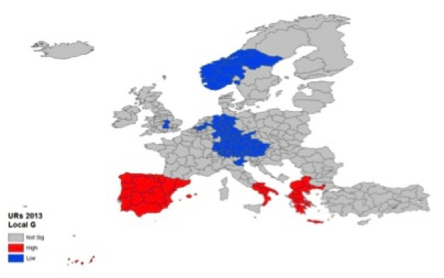
But in 2013, we see very marked spatial divergences in labour market performance. The ‘hot spots’ have enveloped the entire nations of Greece and Spain and most of Southern Italy.

There is high unemployment elsewhere, but the local clusters tell us that the high unemployment in those regions is interlinked with its neighbours which means something systematic is going on – the high unemployment is not random.

Figure 6 G-statistics 2013

High unemployment rates concentrated within specific geographic areas are obviously a concern for policy makers, particularly where this may be leading to the cumulative economic decline and associated adverse social pathologies.

This is particularly the case if these ‘hotspots’ and ‘cold spots’ constitute areas which interact strongly in terms of trade and employment.

In the presence of strong interactions (allowing for other explanatory factors such as residential ‘sorting’ or contextual factors which may also be driving the univariate clustering observed), initial sluggish growth in one region will lead to a drop in economic activity in neighbouring regions, particularly if firms in neighbouring regions rely on sales to residents in the initial region or workers rely on the initial region for jobs.

Firm closures in neighbouring regions may result, unemployment rises, local demand falls further, workers migrate and so and so forth. When such spillovers exist and contribute to the observed similarity in neighbouring values, intervention to address unemployment in a single region of a ‘hotspot’ may have flow on benefits to its neighbours.

Conversely, in the presence of strong spatial dependence, failure to address the causes of unemployment may lead to a quickening of economic decline and an exacerbation of regional inequality, even if national employment growth is strong.

The local analysis of European unemployment confirms two things. Firstly, that there is significant geographic segregation in unemployment outcomes.

Secondly, unemployment hotspots have absorbed whole nations in the case of Greece and Spain and large parts of Italy. This tells us that the crisis and subsequent policy response has been particularly severe.

NOTE: The paper goes on to develop more formal spatial econometric models for analysing the driving factors in these shifting patterns and particulary confronts the so-called structural claims with the more obvious explanation based on a collapse in private spending, which was subsequently exacerbated by the imposition of fiscal austerity.

I will report more when we finish the next stage of the work. The maps will be better in the final paper as well and there will be lots more tables and explanations of things. Today is just a rough sketch.

Anyway, the day in the life of a researcher!

Musical close to the week – Surfin’

After all that, we need some cool guitar playing backed by some of the toughest drum-bass around.

The guitarist (one of my favourites) is Jamaican Ernest Ranglin who is playing his ‘hit’ song Surfin in the Blue Note Club in Tokyo in 2007. The other players are Sly Dunbar (drums), Robbie Shakespeare (bass) (of Sly and Robbie fame), and Monty Alexander (piano).

Ernest Ranglin was one of the stalwart session players at the famous Studio One in Kingston and was an early innovator in what became ska the precursor to rock steady and then reggae. He was one of the first to play the chunking, muffled rythm guitar that now defines reggae guitar playing.

He was 75 years old in this video (now 82 and still going strong).

Thoroughly a good way to end this week’s blogging.

Saturday Quiz

The Saturday Quiz will be back again tomorrow. It will be of an appropriate order of difficulty (-:

That is enough for today!

(c) Copyright 2014 Bill Mitchell. All Rights Reserved.