The Weekend Quiz – October 26-27, 2019 – answers and discussion

Here are the answers with discussion for this Weekend’s Quiz. The information provided should help you work out why you missed a question or three! If you haven’t already done the Quiz from yesterday then have a go at it before you read the answers. I hope this helps you develop an understanding of Modern Monetary Theory (MMT) and its application to macroeconomic thinking. Comments as usual welcome, especially if I have made an error.

Question 1:

A sovereign national government can run a balanced fiscal position over the economic cycle (peak to peak) as long as it accepts that after all the spending adjustments are exhausted that the private domestic balance will only be able to save overall if the external balance is in surplus.

The answer is True.

Note that this question begs the question as to how the economy might get into this situation that I have described using the sectoral balances framework. But whatever behavioural forces were at play, the sectoral balances all have to sum to zero. Once you understand that, then deduction leads to the correct answer.

To refresh your memory the balances are derived as follows. The basic income-expenditure model in macroeconomics can be viewed in (at least) two ways: (a) from the perspective of the sources of spending; and (b) from the perspective of the uses of the income produced. Bringing these two perspectives (of the same thing) together generates the sectoral balances.

To refresh your memory the balances are derived as follows. The basic income-expenditure model in macroeconomics can be viewed in (at least) two ways: (a) from the perspective of the sources of spending; and (b) from the perspective of the uses of the income produced. Bringing these two perspectives (of the same thing) together generates the sectoral balances.

From the sources perspective we write:

(1) GDP = C + I + G + (X – M)

which says that total national income (GDP) is the sum of total final consumption spending (C), total private investment (I), total government spending (G) and net exports (X – M).

Expression (1) tells us that total income in the economy per period will be exactly equal to total spending from all sources of expenditure.

We also have to acknowledge that financial balances of the sectors are impacted by net government taxes (T) which includes all tax revenue minus total transfer and interest payments (the latter are not counted independently in the expenditure Expression (1)).

Further, as noted above the trade account is only one aspect of the financial flows between the domestic economy and the external sector. we have to include net external income flows (FNI).

Adding in the net external income flows (FNI) to Expression (2) for GDP we get the familiar gross national product or gross national income measure (GNP):

(2) GNP = C + I + G + (X – M) + FNI

To render this approach into the sectoral balances form, we subtract total net taxes (T) from both sides of Expression (3) to get:

(3) GNP – T = C + I + G + (X – M) + FNI – T

Now we can collect the terms by arranging them according to the three sectoral balances:

(4) (GNP – C – T) – I = (G – T) + (X – M + FNI)

The the terms in Expression (4) are relatively easy to understand now.

The term (GNP – C – T) represents total income less the amount consumed less the amount paid to government in taxes (taking into account transfers coming the other way). In other words, it represents private domestic saving.

The left-hand side of Equation (4), (GNP – C – T) – I, thus is the overall saving of the private domestic sector, which is distinct from total household saving denoted by the term (GNP – C – T).

In other words, the left-hand side of Equation (4) is the private domestic financial balance and if it is positive then the sector is spending less than its total income and if it is negative the sector is spending more than it total income.

The term (G – T) is the government financial balance and is in deficit if government spending (G) is greater than government tax revenue minus transfers (T), and in surplus if the balance is negative.

Finally, the other right-hand side term (X – M + FNI) is the external financial balance, commonly known as the current account balance (CAD). It is in surplus if positive and deficit if negative.

In English we could say that:

The private financial balance equals the sum of the government financial balance plus the current account balance.

We can re-write Expression (6) in this way to get the sectoral balances equation:

(5) (S – I) = (G – T) + CAB

which is interpreted as meaning that government sector deficits (G – T > 0) and current account surpluses (CAB > 0) generate national income and net financial assets for the private domestic sector.

Conversely, government surpluses (G – T < 0) and current account deficits (CAB < 0) reduce national income and undermine the capacity of the private domestic sector to add financial assets.

Expression (5) can also be written as:

(6) [(S – I) – CAB] = (G – T)

where the term on the left-hand side [(S – I) – CAB] is the non-government sector financial balance and is of equal and opposite sign to the government financial balance.

This is the familiar MMT statement that a government sector deficit (surplus) is equal dollar-for-dollar to the non-government sector surplus (deficit).

The sectoral balances equation says that total private savings (S) minus private investment (I) has to equal the public deficit (spending, G minus taxes, T) plus net exports (exports (X) minus imports (M)) plus net income transfers.

All these relationships (equations) hold as a matter of accounting and not matters of opinion.

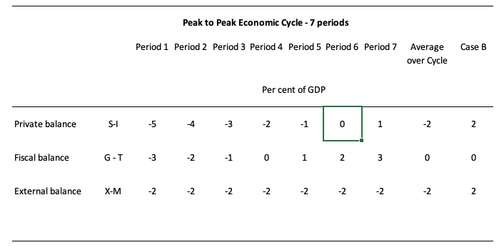
To help us answer the specific question posed, the following Table shows a stylised business cycle with some simplifications. The economy is running a fiscal surplus in the first three periods (but declining) and then increasing deficits.

Over the entire cycle the fiscal balance averages to zero. So the deficits are covered by fully offsetting surpluses over the cycle.

The simplification is the constant external deficit (that is, no cyclical sensitivity) of 2 per cent of GDP over the entire cycle.

You can then see what the private domestic balance is doing clearly. When the fiscal balance is in surplus, the private domestic balance is in deficit – househods and firms are spending more than they are earning overall.

The larger the fiscal surplus the larger the private deficit for a given external deficit.

As the fiscal position moves into deficit, the private domestic balance approaches balance and then finally in Period 6, the fiscal deficit is large enough to offset the demand-draining external deficit (2 per cent of GDP) and so the private domestic sector breaks even. By Period 7 the private domestic sector can save overall because the injection from the deficit is larger than the leakage from the external deficit.

The fiscal deficits underpin spending and allowing income growth to be sufficient to generate savings greater than investment in the private domestic sector.

On average over the cycle, under these conditions (balanced fiscal position) the private domestic deficit exactly equals the external deficit. As a result over the course of the economic cycle, the private domestic sector will become increasingly indebted if this situation persisted.

You can see in the Case B column, which shows average balances over some cycle that when the external position is in surplus, the private domestic sector can save overall even if the fiscal position is balanced at zero.

The following blog posts may be of further interest to you:

• Barnaby, better to walk before we run
• Stock-flow consistent macro models
• Norway and sectoral balances
• The OECD is at it again!

Question 2:

Modern Monetary Theory (MMT) demonstrates that excessive real wages can cause unemployment.

The answer is True.

In this blog – What causes mass unemployment? – I outline the way aggregate demand failures causes of mass unemployment and use a simple two person economy to demonstrate the point.

I also presented the famous Keynes versus the Classics debate about the role of real wage cuts in stimulating employment that was well rehearsed during the Great Depression.

The debate was multi-dimensioned but the role of wage flexibility was a key aspect. In the classical model of employment determination, which remains the basis of mainstream textbook analysis, cuts in the nominal wage will increase employment because it is considered they will reduce the real wage.

The mainstream textbook model assumes that economies produce under the constraint of the so-called diminishing marginal product of labour. So adding an extra worker will reduce productivity because they assume the available capital that workers get to use is fixed in the short-run.

This assertion which does not stack up in the real world, yields the downward sloping marginal product of labour (the contribution of the last worker to production) relationship in the textbook model. Then profit maximising firms set the marginal product equal to the real wage to determine their employment decisions.

They do this because the marginal product is what the last worker produces (at the margin) and the real wage is what the worker costs in real terms to hire.

So when they have screwed the last bit of production out of the last worker hired and it equals the real wage, they have thus made “real gains” on all previous workers employed and cannot do any better – hence, they are said to have maximised profits.
Labour demand is thus inverse to the real wage. As the real wage rises, employment falls in this model because the marginal product falls with employment.

The simplest version is that labour supply in the mainstream model (and complex versions don’t add anything anyway) says that households equate the marginal disutility of work (the slope of the labour supply function) with the real wage (indicating the opportunity cost of leisure) to determine their utility maximising labour supply.

So in English, it is assumed that workers hate work and but like leisure (non-work). They will only go to work to get an income and the higher the real wage the more work they will supply because for each hour of labour supplied their prospective income is higher. Again, this conception is arbitrary and not consistent with countless empirical studies which show the total labour supply is more or less invariant to movements in the real wage.

Other more complex variations of the mainstream model depict labour supply functions with both non-zero real wage elasticities and, consistent with recent real business cycle analysis, sensitivity to the real interest rate. All ridiculous. Ignore them!

In the mainstream model, labour market clearing – that is when all firms who want to hire someone can find a worker to hire and all workers who want to work can find sufficient work – requires that the real wage equals the marginal product of labour. The real wage will change to ensure that this is maintained at all times thus providing the classical model with continuous full employment. So anything that prevents this from happening (government regulations) will create unemployment.

If a worker is “unemployed” then it must mean they desire a real wage that is excessive in relation to their productivity. The other way the mainstream characterise this is that the worker values leisure greater than income (work).

The equilibrium employment levels thus determine via the technological state of the economy (productivity function) the equilibrium (or full employment) level of aggregate supply of real output. So once all the labour markets are cleared the total level of output that is produced (determined by the productivity levels) will equal total output or GDP.

It was of particular significance for Keynes that the classical explanation for real output determination did not depend on the aggregate demand for it at all.

He argued that firms will not produce output that they do not think they will sell. So for him, total supply of GDP must be determined by aggregate demand (which he called effective demand – spending plans backed by a willingness to impart cash).

In the General Theory, Keynes questioned whether wage reductions could be readily achieved and was sceptical that, even if they could, employment would rise.

The adverse consequences for the effective demand for output were his principal concern.

So Keynes proposed the revolutionary idea (at the time) that employment was determined by effective monetary demand for output. Since there was no reason why the total demand for output would necessarily correspond to full employment, involuntary unemployment was likely.

Keynes revived Marx’s earlier works on effective demand (although he didn’t acknowledge that in his work – being anti-Marxist). What determined effective demand? There were two major elements: the consumption demand of households, and the investment demands of business.

So demand for aggregate output determined production levels which in turn determined total employment.

Keynes model reversed the classical causality in the macroeconomy. Demand determined output. Production levels then determined employment based on the current level of productivity. The labour market is then constrained by this level of employment demand. At the current money wage level, the level of unemployment (supply minus demand) is then determined. The firms will not expand employment unless the aggregate constraint is relaxed.

Keynes also argued that in a recession, the real wage might not fall because workers bargain for money or nominal wages, not real wages. The act of dropping money wages across the board would also reduce aggregate demand and prices would also fall. So there was no guarantee that real wages (the ratio of wages to prices) would therefore fall. They may rise or stay about the same.

Falling prices might, however, depress business profit expectations and so cut into demand for investment. This would actually reduce the demand for workers and prevent total employment from rising. The system interacts with itself, and an equilibrium of full employment cannot be achieved within the labour market.

Keynes also claimed that in a recession it should be clear that the problem is not that the real wage is too high, but rather that the prices are too low (as prices fall with lower production).

However, in Keynes’ analysis, attempting to cut real wages by cutting nominal wages would be resisted by the workers because they will not promote higher employment or output and also would imperil their ability to service their nominal contractual commitments (like mortgages). The argument is that workers will tolerate a fall in real wages brought about by prices rising faster than nominal wages because, within limits, they can still pay their nominal contractual obligations (by cutting back on other expenditure).

A more subtle point argued by Keynes is that wage cut resistance may be beneficial because of the distribution of income implications. If real wages fall, the share of real output claimed by the owners of capital (or non-labour fixed inputs) rises. Assuming such ownership is concentrated in a few hands, capitalists can be expected to have a higher propensity to save than the working class.

If so, aggregate saving from real output will increase and aggregate demand will fall further setting off a second round of oversupply of output and job losses.

It is also important to differentiate what happens if a firm lowers its wage level against what happens in the whole economy does the same. This relates to the so-called interdependence of demand and supply curves.

The mainstream model claims that the two sides of the market are independent so that a supply shift will not cause the demand side of the market to shift. So in this context, if a firm can lower its money wage rates it would not expect a major fall in the demand for its products because its workforce are a small proportion of total employment and their incomes are a small proportion of total demand.

If so, the firm can reduce its prices and may enjoy rising demand for its output and hence put more workers on. So the demand and supply of output are independent.

However there are solid reasons why firms will not want to behave like this. They get the reputation of being a capricious employer and will struggle to retain labour when the economy improves. Further, worker morale will fall and with it productivity. Other pathologies such as increased absenteeism etc would accompany this sort of firm behaviour.

But if the whole economy takes a wage cut, then while wage are a cost on the supply side they are an income on the demand side. So a cut in wages may reduce supply costs but also will reduce demand for output. In this case the aggregate demand and supply are interdependent and this violates the mainstream depiction.

This argument demonstrates one of the famous fallacies of composition in mainstream theory. That is, policies that might work at the micro (firm/sector) level will not generalise to work at the macroeconomic level.

There was much more to the Keynes versus the Classics debate but the general idea is as presented.
MMT integrates the insights of Keynes and others into a broader monetary framework. But the essential point is that mass unemployment is a macroeconomic phenomenon and trying to manipulate wage levels (relative to prices) will only change output and employment at the macroeconomic level if changes in demand are achieved as saving desires of the non-government sector respond.

It is highly unlikely for all the reasons noted that cutting real wages will reduce the non-government desire to save.

MMT tells us that the introduction of state money (the currency issued by the government) introduces the possibility of unemployment. There is no unemployment in non-monetary economies. As a background to this discussion you might like to read this blog – Functional finance and modern monetary theory .

MMT shows that taxation functions to promote offers from private individuals to government of goods and services in return for the necessary funds to extinguish the tax liabilities.

So taxation is a way that the government can elicit resources from the non-government sector because the latter have to get $s to pay their tax bills. Where else can they get the $s unless the government spends them on goods and services provided by the non-government sector?

A sovereign government is never revenue constrained and so taxation is not required to “finance” public spending. The mainstream economists conceive of taxation as providing revenue to the government which it requires in order to spend. In fact, the reverse is the truth.

Government spending provides revenue to the non-government sector which then allows them to extinguish their taxation liabilities. So the funds necessary to pay the tax liabilities are provided to the non-government sector by government spending.

It follows that the imposition of the taxation liability creates a demand for the government currency in the non-government sector which allows the government to pursue its economic and social policy program.

The non-government sector will seek to sell goods and services (including labour) to the government sector to get the currency (derived from the government spending) in order to extinguish its tax obligations to government as long as the tax regime is legally enforceable. Under these circumstances, the non-government sector will always accept government money because it is the means to get the $s necessary to pay the taxes due.

This insight allows us to see another dimension of taxation which is lost in mainstream economic analysis. Given that the non-government sector requires fiat currency to pay its taxation liabilities, in the first instance, the imposition of taxes (without a concomitant injection of spending) by design creates unemployment (people seeking paid work) in the non-government sector.

The unemployed or idle non-government resources can then be utilised through demand injections via government spending which amounts to a transfer of real goods and services from the non-government to the government sector.

In turn, this transfer facilitates the government’s socio-economics program. While real resources are transferred from the non-government sector in the form of goods and services that are purchased by government, the motivation to supply these resources is sourced back to the need to acquire fiat currency to extinguish the tax liabilities.

Further, while real resources are transferred, the taxation provides no additional financial capacity to the government of issue.
Conceptualising the relationship between the government and non-government sectors in this way makes it clear that it is government spending that provides the paid work which eliminates the unemployment created by the taxes.

So it is now possible to see why mass unemployment arises. It is the introduction of State Money (defined as government taxing and spending) into a non-monetary economy that raises the spectre of involuntary unemployment.

As a matter of accounting, for aggregate output to be sold, total spending must equal the total income generated in production (whether actual income generated in production is fully spent or not in each period).

Involuntary unemployment is idle labour offered for sale with no buyers at current prices (wages). Unemployment occurs when the private sector, in aggregate, desires to earn the monetary unit of account through the offer of labour but doesn’t desire to spend all it earns, other things equal.

As a result, involuntary inventory accumulation among sellers of goods and services translates into decreased output and employment.

In this situation, nominal (or real) wage cuts per se do not clear the labour market, unless those cuts somehow eliminate the private sector desire to net save, and thereby increase spending.

So we are now seeing that at a macroeconomic level, manipulating wage levels (or rates of growth) would not seem to be an effective strategy to solve mass unemployment.

MMT then concludes that mass unemployment occurs when net government spending is too low.

To recap: The purpose of State Money is to facilitate the movement of real goods and services from the non-government (largely private) sector to the government (public) domain.

Government achieves this transfer by first levying a tax, which creates a notional demand for its currency of issue.

To obtain funds needed to pay taxes and net save, non-government agents offer real goods and services for sale in exchange for the needed units of the currency. This includes, of-course, the offer of labour by the unemployed.

The obvious conclusion is that unemployment occurs when net government spending is too low to accommodate the need to pay taxes and the desire to net save.

This analysis also sets the limits on government spending. It is clear that government spending has to be sufficient to allow taxes to be paid. In addition, net government spending is required to meet the private desire to save (accumulate net financial assets).

It is also clear that if the Government doesn’t spend enough to cover taxes and the non-government sector’s desire to save the manifestation of this deficiency will be unemployment.

Keynesians have used the term demand-deficient unemployment. In MMT, the basis of this deficiency is at all times inadequate net government spending, given the private spending (saving) decisions in force at any particular time.

Shift in private spending certainly lead to job losses but the persistent of these job losses is all down to inadequate net government spending.

But in terms of the question – after all that – it is clear that excessive real wages could impinge on the rate of profit that the capitalists desired and if they translate that into a cut back in investment then aggregate demand might fall. Note: this explanation has nothing to do with the standard mainstream textbook explanation. It is totally consistent with MMT and the Keynesian story – output and employment is determined by aggregate demand and anything that impacts adversely on the latter will undermine employment.

The following blog posts may be of further interest to you:

• Functional finance and modern monetary theory
• What causes mass unemployment?
• Modern monetary theory in an open economy
• Deficit spending 101 – Part 1
• Deficit spending 101 – Part 2
• Deficit spending 101 – Part 3

Question 3:

If workers are to get a larger share of GDP then their wages have to grow faster than inflation.

The answer is False.

The wage share in nominal GDP is expressed as the total wage bill as a percentage of nominal GDP. Economists differentiate between nominal GDP ($GDP), which is total output produced at market prices and real GDP (GDP), which is the actual physical equivalent of the nominal GDP. We will come back to that distinction soon.

To compute the wage share we need to consider total labour costs in production and the flow of production ($GDP) each period.

Employment (L) is a stock and is measured in persons (averaged over some period like a month or a quarter or a year.

The wage bill is a flow and is the product of total employment (L) and the average wage (w) prevailing at any point in time. Stocks (L) become flows if it is multiplied by a flow variable (W). So the wage bill is the total labour costs in production per period.

So the wage bill = W.L

The wage share is just the total labour costs expressed as a proportion of $GDP – (W.L)/$GDP in nominal terms, usually expressed as a percentage. We can actually break this down further.

Labour productivity (LP) is the units of real GDP per person employed per period. Using the symbols already defined this can be written as:

LP = GDP/L

so it tells us what real output (GDP) each labour unit that is added to production produces on average.

We can also define another term that is regularly used in the media – the real wage – which is the purchasing power equivalent on the nominal wage that workers get paid each period. To compute the real wage we need to consider two variables: (a) the nominal wage (W) and the aggregate price level (P).

We might consider the aggregate price level to be measured by the consumer price index (CPI) although there are huge debates about that. But in a sense, this macroeconomic price level doesn’t exist but represents some abstract measure of the general movement in all prices in the economy.

Macroeconomics is hard to learn because it involves these abstract variables that are never observed – like the price level, like “the interest rate” etc. They are just stylisations of the general tendency of all the different prices and interest rates.

Now the nominal wage (W) – that is paid by employers to workers is determined in the labour market – by the contract of employment between the worker and the employer. The price level (P) is determined in the goods market – by the interaction of total supply of output and aggregate demand for that output although there are complex models of firm price setting that use cost-plus mark-up formulas with demand just determining volume sold. We shouldn’t get into those debates here.

The inflation rate is just the continuous growth in the price level (P). A once-off adjustment in the price level is not considered by economists to constitute inflation.

So the real wage (w) tells us what volume of real goods and services the nominal wage (W) will be able to command and is obviously influenced by the level of W and the price level. For a given W, the lower is P the greater the purchasing power of the nominal wage and so the higher is the real wage (w).

We write the real wage (w) as W/P. So if W = 10 and P = 1, then the real wage (w) = 10 meaning that the current wage will buy 10 units of real output. If P rose to 2 then w = 5, meaning the real wage was now cut by one-half.

So the proposition in the question – that nominal wages grow faster than inflation – tells us that the real wage is rising.

Nominal GDP ($GDP) can be written as P.GDP, where the P values the real physical output.

Now if you put of these concepts together you get an interesting framework. To help you follow the logic here are the terms developed and be careful not to confuse $GDP (nominal) with GDP (real):

• Wage share = (W.L)/$GDP
• Nominal GDP: $GDP = P.GDP
• Labour productivity: LP = GDP/L
• Real wage: w = W/P

By substituting the expression for Nominal GDP into the wage share measure we get:

Wage share = (W.L)/P.GDP

In this area of economics, we often look for alternative way to write this expression – it maintains the equivalence (that is, obeys all the rules of algebra) but presents the expression (in this case the wage share) in a different “view”.

So we can write as an equivalent:

Wage share – (W/P).(L/GDP)

Now if you note that (L/GDP) is the inverse (reciprocal) of the labour productivity term (GDP/L). We can use another rule of algebra (reversing the invert and multiply rule) to rewrite this expression again in a more interpretable fashion.

So an equivalent but more convenient measure of the wage share is:

Wage share = (W/P)/(GDP/L) – that is, the real wage (W/P) divided by labour productivity (GDP/L).

I won’t show this but I could also express this in growth terms such that if the growth in the real wage equals labour productivity growth the wage share is constant. The algebra is simple but we have done enough of that already.

That journey might have seemed difficult to non-economists (or those not well-versed in algebra) but it produces a very easy to understand formula for the wage share.

Two other points to note. The wage share is also equivalent to the real unit labour cost (RULC) measures that Treasuries and central banks use to describe trends in costs within the economy. Please read my blog – Saturday Quiz – May 15, 2010 – answers and discussion – for more discussion on this point.

Now it becomes obvious that if the nominal wage (W) grows faster than the price level (P) then the real wage is growing. But that doesn’t automatically lead to a growing wage share. So the blanket proposition stated in the question is false.

If the real wage is growing at the same rate as labour productivity, then both terms in the wage share ratio are equal and so the wage share is constant.

If the real wage is growing but labour productivity is growing faster, then the wage share will fall.

Only if the real wage is growing faster than labour productivity , will the wage share rise.

The wage share was constant for a long time during the Post Second World period and this constancy was so marked that Kaldor (the Cambridge economist) termed it one of the great “stylised” facts. So real wages grew in line with productivity growth which was the source of increasing living standards for workers.

The productivity growth provided the “room” in the distribution system for workers to enjoy a greater command over real production and thus higher living standards without threatening inflation.

Since the mid-1980s, the neo-liberal assault on workers’ rights (trade union attacks; deregulation; privatisation; persistently high unemployment) has seen this nexus between real wages and labour productivity growth broken. So while real wages have been stagnant or growing modestly, this growth has been dwarfed by labour productivity growth.

That is enough for today!

(c) Copyright 2019 William Mitchell. All Rights Reserved.