Analytical appendix for NIPA Chapter 3 – Part 2

I am now using Friday’s blog space to provide draft versions of the Modern Monetary Theory textbook that I am writing with my colleague and friend Randy Wray. We expect to publish the text sometime in 2013. Our (very incomplete) textbook homepage – Modern Monetary Theory and Practice – has draft chapters and contents etc in varying states of completion. Comments are always welcome. Note also that the text I post here is not intended to be a blog-style narrative but constitutes the drafting work I am doing – that is, the material posted will not represent the complete text. Further it will change as the drafting process evolves.

The Table of Contents for the first draft, which is nearly completed, currently lists Chapter 3 as National Income Accounting, with a section 3.7 Using the NIPA Framework to Model the Macro Economy. The status of this section might change but the content aims to present some analytical terminology that is used in the specification of macroeconomic models which the student encounters throughout the textbook.

The section (or subsection) will cover basic algebra, manipulation of equations, solving simple linear models, consideration of graphs, and some essential tools that help an applied macroeconomist assess data trends etc.

Today, I am adding to the material already developed which is currently available as Chapter 3 Draft, Section 3.8.

The snippets I develop here will be integrated into the draft for further assessment. The ambiguity of the numbering reflects the transient status of these sections.

The first part of this section of the text:

• Analytical appendix for NIPA Chapter 3

[CONTINUING FROM HERE]

Graphical depiction of macroeconomic models

We will also express our theories in graphical terms, which are an alternative to mathematical representation. Here are three ways to express the same theoretical idea.

1. Household consumption rises proportionately with disposable income but the proportion is less than one.

2. C = C₀ + cY_d, where 0 < c < 1 and C₀ is a constant (fixed value). The less than sign (<) tells us that the MPC lies between the value of 0 and 1, that is, it is positive but less than 1.

For now, we assume taxes are zero which means that national income (Y) and national disposable income (Y_d) are equal.

3. Graphical form:

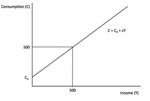
Figure A1 depicts a general consumption function.

Figure A1 Consumption function

If C₀ = 100, and c = 0.8, and Y = 500 then total consumption would be 500. We could have solved the equation C = C₀ + cY by inserting the known values of the parameters and explanatory variable (in this case, income) into the equation and solving it.

Thus:

C = C₀ + cY = 100 + 0.8 x 500 = 500.

You can also see that by tracing a vertical line from where Disposable income equals 500 up to the graph line and then tracing across the vertical axis we derive the value of Consumption by where that line crosses the vertical axis.

The slope of the line is the Marginal Propensity to Consume (c). How do we derive a slope of a line and what does it mean? In Chapter 3 we will deal with applications of the slope of a line when we study the principle of the expenditure multiplier.

To advance our understanding, assume that national income rose to 1000. We know that Consumption would rise to 900.

Check that you can solve the equation C = C₀ + cY = 100 + 0.8 x 1000 = 900.

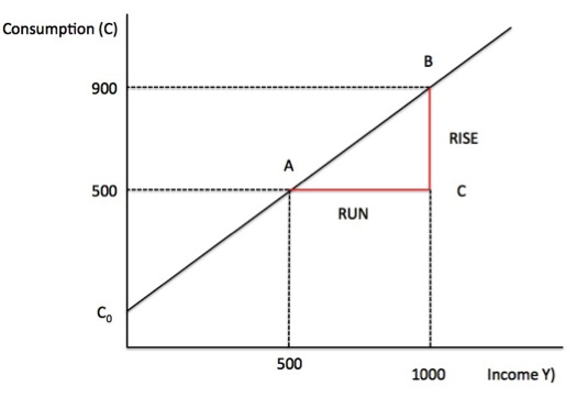
Consider Figure A2 which shows the two combinations of Y and C that we have now determined. The first point, denoted A, represents the combination (Y₁, C₁) = (500, 500).

The second point, denoted B, represents the combination (Y₂, C₂) = (1000, 900).

Figure A2 Slope of Consumption function

We represent the slope of the line that intersects A and B using the following formula:

You can see this is also the ratio of the segments BC/AC or in words “Rise over Run” (the change in C by the change in Y). This rule generalises to any linear function. Note that, depending on the context, Rise could be Fall.

You can check the slope of our consumption function by noting that BC = 400 and AC = 500 so BC/AC = 0.8, which is the Marginal Propensity to Consume (c).

We noted earlier that we usually denote the change in a variable using the Greek symbol Δ. In that context the slope of the consumption function would be c = ΔC/ΔY and that slope would be constant at all points on the function.

The graphical approach to determining the slope of the line is confined to linear equations. If the function is non-linear (for example, a curve), the slope formula we have derived only provides us with the average slope between two points.

A more general approach is required when the relationship of interest is non-linear (for example, a quadratic or cubic function) and the slope is constantly varying.

In this situation, differential calculus is used and the slope of the function at some specific point is defined by the derivative of the function.

For the function, y = f(x), the derivative is typically represented by the expression dy/dx of f'(x).

Note that when deploying differential calculus, we are assuming (using the example above) that ΔY is infinitesimally small (that is, a value approaching zero). Typically, we will be concerned with changes in variables that are larger than this and so the tools of calculus will be of limited use to us in this textbook. Thus, we will use calculus sparingly in the textbook but it is useful to understand the basic concept of a derivative.

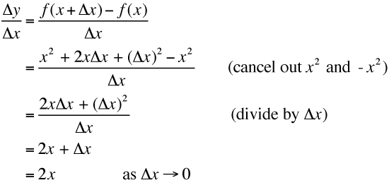
The slope of y = f(x) is Δy/Δx. We can see that Δy = f(x + Δx) – f(x). Now what would happen if Δx was close to zero?

Take a specific example of a non-linear function, y = x². We say that x is raised to the power of two (or squared). You can see that in a linear function such as y = 2x, x is raised to the power of one and we know that x¹ = x.

In f(x) = x², f(x + Δx) = (x + Δx)² = x2 + 2x Δx + (Δx)²

Now if we substitute that into the slope formula we get:

So where y = x², dy/dx = 2x. We say this in English as the derivative of x² is 2x as dx approaches zero.

What does this mean? It means that if y = x², the rate of change at any point is 2x. If x = 4, then the rate of change in y is 8. If x = 5, the rate of change in y is 10.

More generally if y = xⁿ, then dy/dx = nx^n-1. Thus if y = x³, dy/dx = 3x².

In the consumption function C = C₀ + cY, the general formula for a derivative would yield dC/dY = cY^1-1 = cY⁰ = c, which is consistent with what we have already found. Note that Y⁰ = 1.

Power series algebra and the expenditure multiplier

We have introduced the concept of the expenditure multiplier, which we consider further in Chapter X. It allows us to calculate the total change in national income following a change in one of the autonomous components of aggregate demand, such as government spending or private investment.

Multipliers play a central role in discussions of the economic impact of policy interventions. The multiplier depends on the magnitude of the initial injection of expenditure plus the induced expenditure that follows. We will learn that when, for example, the government increases its spending, national income rises by that amount, which, in turn, induces further consumption expenditure.

Thus if $1 was injected into the economy, total income would initially rise by $1. If the marginal propensity to consume was 0.8, then the initial rise in income would induce a rise in consumption of 0.8 x $1 or 80 cents in period 1. This $0.80 rise in spending would further induce a rise in consumption in period 2 of 0.8 x 0.8 or 64 cents and so on.

The multiplier is thus related to the slope of the function and the algebraic notion of a geometric or power series.

Consider a $1 increase in government spending with c representing the marginal propensity to consume and n being the number of periods. Then we could write the multiplier k as:

(A1)      k = 1 + c + c² + c³ + c⁴ + … + cⁿ

The right-hand expression is called a power series.

Note that:

(A2)      ck = c + c² + c³ + c⁴ + c⁵ + cⁿ + … + cⁿ⁺¹

If we subtract (A2) from (A1) we get:

(A3)      k(1 – c) = 1 – cⁿ⁺¹

(A4)      k = (1 – cⁿ⁺¹)/(1 – c)

(A5)      k = 1/(1 – c)

We interpret (A5) as saying that when n is a large number, the value of cⁿ⁺¹ becomes extremely small if 0 < c < 1. That allows us to simply (A4) to (A5). [TO COME - INDEX NUMBERS, DEFLATORS] We recognise that different students have different ways in which they learn and accumulate knowledge. Some prefer the mathematical approach while others prefer the graphical approach. Others still learn better through reading the written word, even though that form of communication is prone to interpretative issues. In that regard, all the essential material in the text will be presented in all three ways (sometimes the mathematics will appear in the Annexe of the relevant chapter sometimes within the main body of the text. Conclusion

I am now going back through the first draft and editing, adding and refining sections.

Saturday Quiz

The Saturday Quiz will be back again tomorrow. It will be of an appropriate order of difficulty (-:

That is enough for today!

(c) Copyright 2013 Bill Mitchell. All Rights Reserved.