The Weekend Quiz – August 31-September 1, 2019 – answers and discussion

August 31, 2019
bill
Saturday quiz
0 Comments

Here are the answers with discussion for this Weekend’s Quiz. The information provided should help you work out why you missed a question or three! If you haven’t already done the Quiz from yesterday then have a go at it before you read the answers. I hope this helps you develop an understanding of modern monetary theory (MMT) and its application to macroeconomic thinking. Comments as usual welcome, especially if I have made an error.

Question 1:

The private domestic sector can save overall, even if the government fiscal balance is in surplus, as long as net exports are positive.

The answer is False.

This is a question about the relative magnitude of the sectoral balances – the government fiscal balance, the external balance and the private domestic balance. The balances taken together always add to zero because they are derived as an accounting identity from the national accounts. The balances reflect the underlying economic behaviour in each sector which is interdependent – given this is a macroeconomic system we are considering.

To refresh your memory the sectoral balances are derived as follows. The basic income-expenditure model in macroeconomics can be viewed in (at least) two ways: (a) from the perspective of the sources of spending; and (b) from the perspective of the uses of the income produced. Bringing these two perspectives (of the same thing) together generates the sectoral balances.

From the sources perspective we write:

GDP = C + I + G + (X – M)

which says that total national income (GDP) is the sum of total final consumption spending (C), total private investment (I), total government spending (G) and net exports (X – M).

Expression (1) tells us that total income in the economy per period will be exactly equal to total spending from all sources of expenditure.

We also have to acknowledge that financial balances of the sectors are impacted by net government taxes (T) which includes all taxes and transfer and interest payments (the latter are not counted independently in the expenditure Expression (1)).

Further, as noted above the trade account is only one aspect of the financial flows between the domestic economy and the external sector. we have to include net external income flows (FNI).

Adding in the net external income flows (FNI) to Expression (2) for GDP we get the familiar gross national product or gross national income measure (GNP):

(2) GNP = C + I + G + (X – M) + FNI

To render this approach into the sectoral balances form, we subtract total taxes and transfers (T) from both sides of Expression (3) to get:

(3) GNP – T = C + I + G + (X – M) + FNI – T

Now we can collect the terms by arranging them according to the three sectoral balances:

(4) (GNP – C – T) – I = (G – T) + (X – M + FNI)

The the terms in Expression (4) are relatively easy to understand now.

The term (GNP – C – T) represents total income less the amount consumed less the amount paid to government in taxes (taking into account transfers coming the other way). In other words, it represents private domestic saving.

The left-hand side of Equation (4), (GNP – C – T) – I, thus is the overall saving of the private domestic sector, which is distinct from total household saving denoted by the term (GNP – C – T).

In other words, the left-hand side of Equation (4) is the private domestic financial balance and if it is positive then the sector is spending less than its total income and if it is negative the sector is spending more than it total income.

The term (G – T) is the government financial balance and is in deficit if government spending (G) is greater than government tax revenue minus transfers (T), and in surplus if the balance is negative.

Finally, the other right-hand side term (X – M + FNI) is the external financial balance, commonly known as the current account balance (CAD). It is in surplus if positive and deficit if negative.

In English we could say that:

The private financial balance equals the sum of the government financial balance plus the current account balance.

We can re-write Expression (6) in this way to get the sectoral balances equation:

(5) (S – I) = (G – T) + CAB

which is interpreted as meaning that government sector deficits (G – T > 0) and current account surpluses (CAB > 0) generate national income and net financial assets for the private domestic sector.

Conversely, government surpluses (G – T < 0) and current account deficits (CAB < 0) reduce national income and undermine the capacity of the private domestic sector to add financial assets.

Expression (5) can also be written as:

(6) [(S – I) – CAB] = (G – T)

where the term on the left-hand side [(S – I) – CAB] is the non-government sector financial balance and is of equal and opposite sign to the government financial balance.

This is the familiar MMT statement that a government sector deficit (surplus) is equal dollar-for-dollar to the non-government sector surplus (deficit).

The sectoral balances equation says that total private savings (S) minus private investment (I) has to equal the public deficit (spending, G minus taxes, T) plus net exports (exports (X) minus imports (M)) plus net income transfers.

All these relationships (equations) hold as a matter of accounting and not matters of opinion.

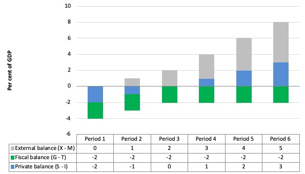
The following graph with accompanying data table lets you see the evolution of the balances expressed in terms of percent of GDP.

In each period I just held the fiscal balance at a constant surplus (2 per cent of GDP) (green bars). Not (G – T) = – 2 means a surplus because T > G.

This is is artificial because as economic activity changes the automatic stabilisers would lead to endogenous changes in the fiscal balance. But we will just assume there is no change for simplicity. It doesn’t violate the logic.

To aid interpretation remember that (S – I ) < 0 means that the private domestic sector is spending more than they are earning; and (X – M) > 0 means the external position is in surplus because imports are greater than exports.

If the nation is running an external surplus it means that the contribution to aggregate spending from the external sector is positive – that is, the net addition to spending would increase output and national income.

A fiscal surplus means the government is spending less than it is draining out of the economy via taxes, which introduces a drag on aggregate spending and constrains the ability of the economy to grow. So the question is what are the relative magnitudes of the external add and the fiscal balance subtract from income?

In Period 1, there is an external balance (X – M = 0) and then for each subsequent period the external balance goes into surplus incrementing by 1 per cent of GDP each period (light-gray bars).

You can see that in the first two periods, private domestic saving is negative, then as the demand injection from the external surplus offsets the fiscal drag arising from the fiscal surplus, the private domestic sector breakeven (spending as much as they earn, so I – S = 0).

Then the demand add overall arising from the net positions of the external and public sectors is positive and the income growth would allow the private sector to save. That is increasingly so as the net demand add increases with the increasing external surplus.

The following blog posts may be of further interest to you:

Question 2:

There is talk among central bankers of renewed programs of quantitative easing to fight off fears of recession as a result of the trade tensions. Fiscal stimulus is also being proposed. The two work in different ways but have the same ultimate impact on net worth in the non-government sector.

The answer is False.

Quantitative easing involves the central bank buying assets from the non-government sector – government bonds and high quality corporate debt.

The central bank is doing is swapping financial assets with the banks – they sell their financial assets and receive back in return extra reserves.

This the central bank is buying one type of financial asset (private holdings of bonds, company paper) and exchanging it for another (reserve balances at the central bank). The net financial assets in the private sector are in fact unchanged although the portfolio composition of those assets is altered (maturity substitution) which changes yields and returns.

In terms of changing portfolio compositions, quantitative easing increases central bank demand for ‘long maturity’ assets held in the private sector which reduces interest rates in this maturity segment of the yield curve. These are traditionally thought of as the investment rates.

This might increase aggregate demand given the cost of investment funds is likely to drop. But on the other hand, the lower rates reduce the interest-income of savers who will reduce consumption (demand) accordingly.

How these opposing effects balance out is unclear but the evidence suggests there is not very much impact at all.

Fiscal policy adds net financial assets to the non-government sector by way of contradistinction to QE.

The following blog posts may be of further interest to you:

Question 3:

While continuous national governments deficits are possible if the non-government sector desires to save overall, they do imply continuously rising public debt levels as a percentage of GDP (under current debt-issuance arrangements).

The answer is False.

While Modern Monetary Theory (MMT) places no particular importance in the public debt to GDP ratio for a sovereign government, given that insolvency is not an issue, the mainstream debate is dominated by the concept. The unnecessary practice of fiat currency-issuing governments of issuing public debt $-for-$ to match public net spending (deficits) ensures that the debt levels will always rise when there are deficits.

But the rising debt levels do not necessarily have to rise at the same rate as GDP grows. The question is about the debt ratio not the level of debt per se.

Rising deficits often are associated with declining economic activity (especially if there is no evidence of accelerating inflation) which suggests that the debt/GDP ratio may be rising because the denominator is also likely to be falling or rising below trend.

Further, historical experience tells us that when economic growth resumes after a major recession, during which the public debt ratio can rise sharply, the latter always declines again.

It is this endogenous nature of the ratio that suggests it is far more important to focus on the underlying economic problems which the public debt ratio just mirrors.

The mainstream textbooks are full of elaborate models of debt pay-back, debt stabilisation etc which all claim (falsely) to “prove” that the legacy of past deficits is higher debt and to stabilise the debt, the government must eliminate the deficit which means it must then run a primary surplus equal to interest payments on the existing debt.

A primary fiscal balance is the difference between government spending (excluding interest rate servicing) and taxation revenue.

The standard mainstream framework, which even the so-called progressives (deficit-doves) use, focuses on the ratio of debt to GDP rather than the level of debt per se.

The following equation captures the approach:

So the change in the debt ratio is the sum of two terms on the right-hand side: (a) the difference between the real interest rate (r) and the GDP growth rate (g) times the initial debt ratio; and (b) the ratio of the primary deficit (G-T) to GDP.

The real interest rate is the difference between the nominal interest rate and the inflation rate.

This standard mainstream framework is used to highlight the dangers of running deficits. But even progressives (not me) use it in a perverse way to justify deficits in a downturn balanced by surpluses in the upturn.

Many mainstream economists and a fair number of so-called progressive economists say that governments should as some point in the business cycle run primary surpluses (taxation revenue in excess of non-interest government spending) to start reducing the debt ratio back to “safe” territory.

Almost all the media commentators that you read on this topic take it for granted that the only way to reduce the public debt ratio is to run primary surpluses. That is what the whole “credible exit strategy” rhetoric is about and what is driving the austerity push around the world at present.

So the question is whether continuous national governments deficits imply continuously rising public debt levels as a percentage of GDP. While MMT advocates running fiscal deficits when they are necessary to fill a spending gap left by non-government saving, it does not tell us that a currency-issuing government running a deficit can never reduce the debt ratio.

The standard formula above can easily demonstrate that a nation running a primary deficit can reduce its public debt ratio over time.

Furthermore, depending on contributions from the external sector, a nation running a deficit will more likely create the conditions for a reduction in the public debt ratio than a nation that introduces an austerity plan aimed at running primary surpluses.

Here is why that is the case. A growing economy can absorb more debt and keep the debt ratio constant or falling.

Even with an increasing (or unchanged) deficit, real GDP growth can reduce the public debt ratio, which is what has happened many times in past history following economic slowdowns.

Economists like Krugman and Mankiw argue that the government could (should) reduce the ratio by inflating it away. Noting that nominal GDP is the product of the price level (P) and real output (Y), the inflating story just increases the nominal value of output and so the denominator of the public debt ratio grows faster than the numerator.

But stimulating real growth (that is, in Y) is the other more constructive way of achieving the same relative adjustment in the denominator of the public debt ratio and its numerator.

But the best way to reduce the public debt ratio is to stop issuing debt. A sovereign government doesn’t have to issue debt if the central bank is happy to keep its target interest rate at zero or pay interest on excess reserves.

The discussion also demonstrates why tightening monetary policy makes it harder for the government to reduce the public debt ratio – which, of-course, is one of the more subtle mainstream ways to force the government to run surpluses.

The following blog may be of further interest to you: