The recent extreme weather in the northern hemisphere, the twin monster tropical storms in Japan,…
The distinguished economists just embarrass themselves
People are allowed to change their opinions or assessments in the light of new evidence. Diametric changes of position are fine and one should not be pilloried for making such a shift in outlook. Quite the contrary. But when the passage of time reveals that a person just recites the same litany despite being continually at odds with the evidence, then that person’s view should be disregarded, notwithstanding the old saying that a defunct clock is correct twice in each 24 hours. The US Congressional Budget Office (CBO) released its latest – The Budget and Economic Outlook: 2018 to 2028 (April 9, 2018) – and various commentators and media outlets have gone into conniptions over it. The economists that have responded – and they come with affiliations from both sides of US politics (although it is hard to differentiate separate ‘sides’ in the US anymore such is the demise of the Democrat Party) – have significantly embarrassed themselves. Their hysteria is not matched with the facts and they have been guilty of invoking these hysterical responses year-in, year-out for many years. A crack in a record, goes click, click, click, click and repeats ad infinitum. Sort of like the nonsensical arguments about US fiscal deficits that have appeared in the US press this last week.
The CBO Report
The full CBO report is available – HERE.
The CBO exercise is to assume “that current laws governing taxes and spending generally remain unchanged” and then project what that means for economic growth, the fiscal balance and the evolution of public debt over the forecast horizon.
The basic conclusions were:
1. “potential and actual real GDP are projected to grow more quickly over the next few years … because of recently enacted legislation … Over the next decade, the unemployment rate is lower …” That all sounds positive as long as the growth is sustainable in environmental terms.
2. “CBO estimates that the 2018 deficit will total $804 billion, $139 billion more than the $665 billion shortfall recorded in 2017”, which relates directly to conclusion 1. Higher deficits at a time when private spending growth is modest will typically increase capacity utilisation and reduce unemployment.
3. “In CBO’s projections, budget deficits continue increasing after 2018, rising from 4.2 percent of GDP this year to 5.1 percent in 2022 … Deficits remain at 5.1 percent between 2022 and 2025 before dipping at the end of the period … Over the 2021-2028 period, projected deficits average 4.9 percent of GDP …”
And so with current account deficits on-going and draining growth, the rising deficit allows the private domestic sector to reduce its debt exposure by increasing its overall saving without damaging over economic growth.
The CBO claim that the 5.1 per cent of GDP deficits “has been exceeded in only five years since 1946; four of those years followed the deep 2007-2009 recession” as if there is something alarming about that.
But it is highly significant in my view that in the – Data Underlying Figures – and hence the analysis, there is no mention of the current account position of the US, as if it is irrelevant in assessing the appropriateness of the fiscal stance.
I could write a lot about the underlying modelling techniques and certainly come up with different estimates to the CBO. But really that is not the important point.
In general, the CBO’s neoliberal bias will lead them to understate the degree of slack in the economy and overstate the structural component of the fiscal balance.
But that is not what I want to consider in this blog post.
Hysterical responses
The response from commentators has been largely hysterical.
In the lead up to the release of the CBO analysis, a so-called “group of distinguished economists from the Hoover Institution” (Source) – (the distinguished reflecting a state where the English language loses all meaning) – wrote an Op Ed for the Washington Post (March 27, 2018) – A debt crisis is on the horizon.
I guess this was a cut and paste job from stuff this lot (Boskin, Cochrane, Cogan, Shultz and Taylor) have been writing and mouthing for years now.
The authors peddle out the same old predictions:
1. Noting the future could be bright (AI, 3D printing, medical advances, etc), they conclude that “a major obstacle stands squarely in the way of this promise: high and sharply rising government debt”.
2. “For years, economists have warned of major increases in future public debt burdens. That future is on our doorstep” – okay, time is up. It was up many years ago but that doorstep is now forgotten. It has shifted to now.
3. Then the usual take a figure and divide it by the known population and attribute responsibility:
Unless Congress acts to reduce federal budget deficits, the outstanding public debt will reach $20 trillion a scant five years from now, up from its current level of $15 trillion. That amounts to almost a quarter of million dollars for a family of four, more than twice the median household wealth.
4. Then add the “unprecedented in U.S. history” angle.
5. Then lie about causality: “In recent months, we have seen an inevitable rise in interest rates from their low levels of recent years.”
6. Then infer that “treasury debt holders … [will] … start to doubt our government’s ability to repay, or to attract future lenders, they will demand higher interest rates to compensate for the risk.”
They have said that many times but their predictions fail to materialise.
It might be that US treasury bond yields will rise as investors start spreading their portfolios across riskier assets.
But I doubt you would find one serious fixed income investor in the US who believed that the US government was about to default now or later.
7. “More borrowing puts more upward pressure on interest rates, and the spiral continues” – and, as we will see, yields are falling in the US and remain low.
8. Then, do some ridiculous high-school arithmetic as if it is important and draw spurious conclusions:
If, for example, interest rates were to rise to 5 percent, instead of the Trump administration’s prediction of just under 3.5 percent, the interest cost alone on the projected $20 trillion of public debt would total $1 trillion per year. More than half of all personal income taxes would be needed to pay bondholders. Such high interest payments would crowd out financing of needed expenditures to restore our depleted national defense budget, our domestic infrastructure and other critical government activities.
Noting that the interest payments constitute income to the non-government sector.
But the idea that they would financially compromise other components of spending (health, defense, infrastructure etc) is false.
They might in political terms if the views of Taylor and Co were taken seriously. But there is no financial imperative to cut such spending just because income flows to the non-government sector rise.
If the economy hit full capacity (and as we will see below it isn’t close), then the rising interest payments might require the government adjust the composition of its net fiscal outlays somewhat, after some of the stimulus would be lost to rising imports.
But that is a different story altogether to the one being pushed in the Washington Post article.
9. Put it altogether and predict “the specter of a crisis”, which will come “without warning, like an earthquake, as short-term bondholders attempt to escape fiscal carnage”.
And what are these bond-holders actually going to do?
Sell them and take capital losses? Sell them to whom?
And if the bid-to-cover ratios fall on public auctions what do you think will happen then, should the government assess that as being a dangerous situation?
Oh that – the central bank just buys up public debt and controls yields and the treasury spends on. Just like has been done many times in the past.
And the bond-holders – the recipients of corporate welfare – are they really going to walk the plank just because Taylor and Co think they should? Not likely.
10. Finally, use all this spurious assertion to get to the political point they want to make – which the likes of these characters have been making for decades – attack “entitlement spending”.
Yes, social security and medical support for low income earners etc – the US has to get rid of that and rely on the private market for this sort of stuff.
And we know what that would lead to.
Given the respective ages of these authors, I could go back 40 or 50 years in some cases and we would find similar claims being made by one or more of these characters.
A record stuck is a record stuck.
First, these economists failed to see what was happening prior to the GFC.
This was an interview with John B. Taylor (one of the authors of the Washington Post article cited above) from June 2006.
Taylor spoke about the way the IMF has matured to be a more “rule driven” organisation:
And I think that’s one of the reasons people are saying, “What’s the IMF doing? Are they going into obscurity?” Well, they don’t have to do much now because, fortunately, these crises have diminished. As a result, we are moving into a period where people are wondering what the IMF is for.
He then got onto the idea of that the world institutions had finally been able to contain “contagion” when a local crisis occurred.
He said the Asian crisis had “caused a lot of damage” but:
But look at what happened after Argentina defaulted in 2001, and you see there’s no similar jump in spreads anywhere around the world. So it’s a huge difference.
The question is whether it is a lasting phenomenon. I’ve thought a lot about it and written about it. And I think it is a lasting difference. One reason is the more predictable response of the IMF. Second, country policies are better … better monetary policy and fiscal policy. So the policies in a lot of countries are better, and that’s the surest way to stop the contagion. And then finally, I think investors are discriminating more between countries. They don’t automatically think there’s a problem in one country when they see another having a problem.
Then on the long boom:
As for the “Long Boom,” I think I first defined it in the April 1998 Homer Jones lecture that I gave at the St. Louis Fed called “Monetary Policy and the Long Boom.” In that lecture, the empirical phenomenon that I focused on was that the size of fluctuations in the economy has diminished substantially. If you looked back to 1982 from at that time-1997 was the last completed year-you saw what looked like a long boom. You had just one historically very small and short recession-in 1991. So the 15 years from 1982 to 1997 were like a long boom. I asked the question, What was the long boom due to? And I gave the answer that it was monetary policy. I documented how monetary policy had changed since the bad old days of frequent recessions. As long as monetary policy stayed on track, I argued, the long boom would continue.
And the long boom has continued … And now maybe we’re in one that will be even longer, but that will depend on keeping with the good policies. So this phenomenon of long, strong expansions and short, small recessions was how I defined the long boom. The same phenomenon is now called the Great Moderation, and there is continuing debate about its causes. I continue to point to the role of monetary policy in making the Long Boom, or the Great Moderation, happen. I think there really is something to that.
I could have accessed similar quotes from countless economists who during the pre-GFC period extolled the virtues of self-regulated markets, passive fiscal policy (austerity bias) and inflation-targetting monetary policy.
One year after Taylor was claiming that as long as governments held to their policy stances the long boom would continue the GFC hit? It was easy to see the crash coming but Taylor and his colleagues had disappeared up their own hubris.
They didn’t see the crisis coming because their economic theories did not allow them to see the way the sectoral balances were emerging and the rising private sector indebtedness and increased financial risk. Any commentator that dared challange this ‘new macroeconomic consensus’ was vilified by the Groupthink within mainstream economics.
More recently, just as the GFC was unfolding, Taylor was a leading critic of the US stimulus packages. He hadn’t learned a thing.
On August 31, 2009, he wrote an Op Ed in the New York Daily – The Coming Debt Debacle – that the:
These large deficits represent a systemic risk to the economy … Without spending discipline, damaging tax increases are required to close such deficits … The deficits would also bring a long painful period of high inflation like the late 1960s and 1970s, a period of frequent recessions and persistently high unemployment when people began to lose confidence in the dollar.
His view was representative of the academic noise at the time.
John Cochrane from Chicago University is another serial offender. Several times after the GFC manifested, Cochrane popped up in the popular debate extolling what he claimed are the dangers of deficits.
He often predicted rising interest rates; rising, then out-of-control inflation would soon hit the US economy.
In this blog post – How many more experiments do we need (June 21, 2011) – I considered Cochrane’s argument that fiscal stimulus would drive a dangerous inflationary spiral. It was one of many such articles that has fallen foul of the evidence.
See also this blog post – Accelerating inflation has to be out there somewhere … in the dark or somewhere (September 27, 2011) – where John Cochrane is again warning us of “substantial inflation” breakouts in the “in the next few years” as a result of the deficits.
We are now in the seven years out from those predictions and lots of ‘money’ has been injected into various economies and inflation is benign.
There may be supply-side inflation pressures introduced as a result of energy price manipulation but that is not the type of danger that John Cochrane and his ilk are or were predicting.
So how would we assess the current statements? Should we consider their theories that lead to these predictions as being an adequate guide to the future when they failed to predict and understand the biggest economic event in most of our lives?
Answer: they should be disregarded totally.
Then comes the response from economists aligned with the Democrats.
On April 8, 2018, the Washington Post published this response to the Taylor and Co article – A debt crisis is coming. But don’t blame entitlements.
Yes, the title really summarises the argument presented.
We read that the Democrat-aligned economists (Baily, Furman, Krueger, Tyson and Yellen) agree with Taylor and Co that their is “a serious problem” and:
… ever-rising debt and deficits will cause interest rates to rise, and the portion of tax revenue needed to service the growing debt will take an increasing toll on the ability of government to provide for its citizens and to respond to recessions and emergencies.
None of that is in dispute.
These economists have been senior advisors to Democrat presidents in the past and in Yellen’s case the outgoing central bank governor.
They have influence when Democrats control things.
And they demonstrate exactly why a bounder like Donald Trump, a man totally unsuited to take the highest office in the US, was able to be elected.
They demonstrate exactly why the Democratic Party cannot even beat Trump and why the public debate in the US is so asinine.
All of the Taylor and Co. claims are in dispute. None of them are correct.
The ‘Democrat economists’ are incapable of making any contest and are content to use their access to a leading US newspaper to dilly dally around the edges.
Oh, entitlements are just a bit of the problem sort of arguments.
We need smaller deficits but Trump is wrong to make tax cuts now because “The economy was already at or close to full employment and did not need a boost”.
And all that sort of wishy-washy nonsense that neoliberal progressives make (yes, this cohort exists – they mouth some progressive social policies but are deep-down neoliberal when it comes to economics).
Sectoral Balances
Lets start with the sectoral balances, which helps us in understanding the implications of various macroeconomic policy shifts.
For a detailed discussion of the derivation of the balances, please read the blog post – Flow-of-funds and sectoral balances (November 24, 2015).
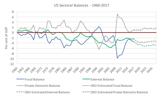
The following graph shows the annual sectoral balances from 1960 to 2017. I then used the CBO’s projections from 2018 to 2028 to extrapolate the balances out to 2028 (the dotted segments):
1. Blue line – Government fiscal balance as a percent of GDP.
2. Green line – External balance as a percent of GDP.
3. Grey line – Private domestic balance as a percent of GDP.
The facts are obvious.
1. The US has a persistent and fairly stable current account deficit of around 2.5 to 3 per cent. CBO does not expect that to change very much.
2. The fiscal retreat in the recent years saw the private domestic balance shrink to nearly zero.
3. The projected movement in the fiscal state allows the private domestic sector to save overall and provides the conditions for that sector to start reducing its massive debt exposure, which, after all, was the cause of the GFC.
4. If the fiscal deficit falls below the current account deficit then the private domestic sector starts to dissave overall – spend more than it earns and starts accumulating increased debt.
5. From the graph, there is not much leeway before that private domestic sector overall leveraging starts to occur, given the size of the external balance.
6. The on-going fiscal deficit is thus not only underpinning growth but also allowing the private domestic sector to deleverage its financial position (save overall).
When the likes of Taylor and Co demand fiscal surpluses they are simultaneously (but not saying) demanding that the private sector debt position increases and that sector dissaves overall.
That is not a sustainable position and would lead to a renewed crisis.
Capacity Utilisation
The Federal Reserve Bank publishes a monthly data series – Industrial Production and Capacity Utilization – G.17 – which provides an indication of how much of the non-labour productive capacity is being utilised.
They define “Capacity utilization for Total Industry (TCU)” as:
… the percentage of resources used by corporations and factories to produce goods in manufacturing, mining, and electric and gas utilities for all facilities located in the United States (excluding those in U.S. territories). We can also think of capacity utilization as how much capacity is being used from the total available capacity to produce demanded finished products …
the capacity index tries to conceptualize the idea of sustainable maximum output, which is defined as the highest level of output a plant can sustain within the confines of its resources … The capacity utilization rate can also implicitly describe how efficiently the factors of production (inputs in the production process) are being used … It sheds light on how much more firms can produce without additional costs. Additionally, this rate gives manufacturers some idea as to how much consumer demand they will be able to meet in the future.
Clearly, when capacity utilisation rates are high, the inflation risk from demand side pressures (that is, spending pressures) increases.
Firms, typically, keep some spare capacity in reserve as a normal strategy so that they can meet unexpected spikes in demand without losing market share. So what might be considered a normal full capacity load will be less than 100 per cent.
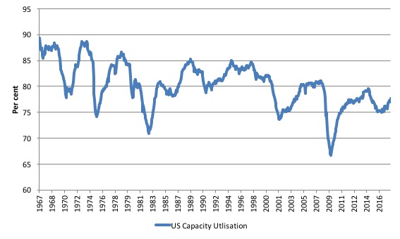
In fact, the average rate of capacity utilisation since this data series was first published in January 1967 has been 80.3 per cent, although the mean rates were much higher in the 1960s and 1970s, before the Monetarist (neo-liberal) era started suppressing growth rates.
The following graph charts the evolution of this data series from January 1967 to February 2018. You can clearly see the cyclical swings associated with recessions.
It is interesting to note that each subsequent recovery since the 1990s has levelled off below the previous level, which is consistent with the observation that the neo-liberal era has been associated with stifled growth rates and elevated levels of excess capacity.
But even in the current recovery, capacity utilisation rates are still below 80 per cent and over the last few months have been heading south again, indicating that firms have increased idle equipment and machinery and plenty of non-inflationary capacity available to meet increased spending growth.
Since Trump was elected the capacity utilisation rate has moved up marginally from 75.4 per cent to 77.6 per cent in February 2019.
It is still well below the most recent peaks.
The conclusion is that there is ample productive capacity in situ to handle the current levels of spending and output without any need to expand productive capacity.
Inflation and inflationary expectations
If the arguments presented in the two cited Washington Post articles were to be treated seriously then we should already sese inflationary expectations pushing up quickly – and they should have done some several years ago.
The Federal Reserve Bank of Cleveland provides the most current series on inflationary expectations and the real interest rate that is available.
In October 2009, the Bank released a discussion paper outlining – A New Approach to Gauging Inflation Expectations. It is a non-technical version of this 2011 paper – Inflation Expectations, Real Rates, and Risk Premia: Evidence from Inflation Swaps.
The latest data from the US Federal Reserve Bank of Cleveland released yesterday (April 11, 2018) – Inflation Expectations – suggest that the:
… latest estimate of 10-year expected inflation is 1.98 percent. In other words, the public currently expects the inflation rate to be below 2 percent on average over the next decade.
This is hardly a sign that the ‘market’ expects inflation to accelerate in the next decade.
The three major rounds of QE in the US were dated as follows:
- Quantitative Easing 1 (QE1, December 2008 to March 2010) – This was announced on November 25, 2008. The program was expanded on March 18, 2009 as described in this FOMC press release.
- Quantitative Easing 2 (QE2, November 2010 to June 2011) – The FOMC announced on – On November 3, 2010 – that it “intends to purchase a further $600 billion of longer-term Treasury securities by the end of the second quarter of 2011, a pace of about $75 billion per month.”
- Quantitative easing 3 (QE3, September 2012 and expanded on December 2012 and terminated in October 2014) – The FOMC announced on – September 13, 2012 – that it “agreed today to increase policy accommodation by purchasing additional agency mortgage-backed securities at a pace of $40 billion per month”. This would continue “If the outlook for the labor market does not improve substantially”. This phase was expanded on – December 12, 2012 – such that the FOMC “will purchase longer-term Treasury securities … initially at a pace of $45 billion per month”. QE was terminated in the US in October 2014.
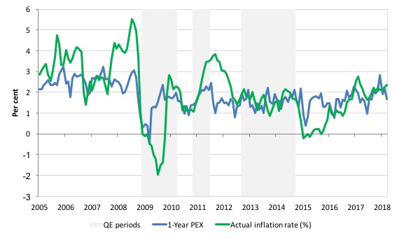
Those phases are depicted by the shaded areas in the following graphs.
The graphs show the evolution of inflationary expectations (PEX) and the actual annual inflation rate from January 2005 to April 2018.
The first graph shows the one-year ahead inflationary expectation while the second shows the expectation over the 10-year horizon (in other words, what people in the US think inflation will be over the next decade).
It is hard to mount an argument that the QE episodes or the sustained fiscal deficit have increased inflationary expectations in any significant manner.
The last phase (QE3) didn’t alter short- or long-run inflationary expectations one iota – they remain low and anchored despite the massive increase in the asset-side of the Federal Reserve balance sheet and the commensurate swelling of bank reserves.
And despite the fiscal deficit increase that has been predicted for some months now.
1-year ahead inflationary expectations
10-year ahead inflationary expectations
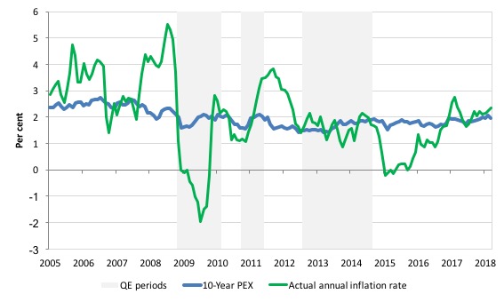
The graphs are interesting because they show that long-term inflationary expectations have remain fairly stable around the Federal Reserve’s 2 per cent anchor.
Even during the early years of the crisis, when the actual inflation rate fell sharply to negative territory, the long term inflationary expectations were stable around the US Federal Reserve’s implicit inflation target.
The shorter term expectations which pick up a lot of the month to month fluctuations in energy and housing prices etc were much more volatile and followed the actual inflation path.
There has been no clear break in behaviour of the long term series since downturn in both the recession and recovery phases.
This suggests that market participants despite all the noise coming from the conservatives judged that growth would return given the fiscal stimulus and realised that QE would do very little in that regard.
They thus judged that the long-term trajectory of the price level would not be distorted by these policy interventions and the different growth experience over the last 7 years.
Taylor and Co and their Democrat partners in the deception are just plain misguided on this matter.
Their arguments have no credibility.
Bond yields
So what about bond yields? Taylor and Co and the neoliberal Democrats both claim that yields would rise given the ongoing and rising fiscal deficit because market participants will lose faith in the capacity of the government to repay the debt.
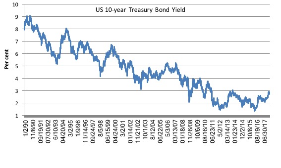
The following graph shows the daily 10-year US Treasury yields from early 1990 to April 10, 2018.
Despite the on-going fiscal deficits, yields have fallen rather dramatically reflecting the increased demand in the bond markets for government bonds (as safe havens).
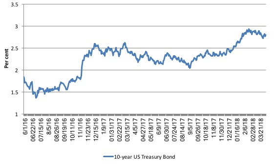
To give a closer view, the next graph shows the same yield from the beginning of 2016 to April 10, 2018. As the US economy has recovered, private portfolio diversification into riskier private assets has seen a small increase in yields.
But even with the knowledge of the increased deficits, the ‘markets’ have increased their demand for 10-year Treasury bonds and the yields have started falling again as a consequence.
There is absolutely no evidence that the fiscal deficits have resulted in rising yields.
Let us be absolutely clear:
1. The private bond markets have no power to stop a currency-issuing government spending.
2. The private bond markets have no power to stop a currency-issuing government running deficits.
3. The private bond markets have no power to set interest rates (yields) if the central bank chooses otherwise.
4. Sovereign governments always rule over bond markets – full stop.
I examine this in more detail in this blog post – The bond vigilantes saddle up their Shetland ponies – apparently (February 18, 2018).
Conclusion
While I would not support the increased US fiscal deficits under current policy proposals from Donald Trump, I would welcome increased deficits if the policy mix was skewed towards introducing a Job Guarantee, improving public infrastructure, expanding the welfare support and improving schools and hospitals.
It is not the deficit or the public debt I would be worried about.
But that is a different discussion to the rabid hysterics that Taylor and Co and their Democrat rivals have engaged in over the last week or so.
Their arguments carry no credibility at all.
That is enough for today!
(c) Copyright 2018 William Mitchell. All Rights Reserved.
Dear Bill
You assume that the current-account deficit of the US is a given, but isn’t there some relation between the current account and the government sector? T + S + M = G + I + X. Well, if T goes up, won’t M and S go down? If G goes up, can’t M and S go up as well? If (G -T) goes up, households have higher disposable income, so they can import more and save more. Conversely, if (G – T) goes down, disposable income of households will decrease, so they may import less and also save less.
Regards. James
Taylor believes that his so-called long boom is due to monetary policy, does he, and he thinks we’re in one now. OMFG! He lives on Planet Zog.
Your blog post about sectoral balances that you cite has you include a tweet by Ann Pettifor where she indicates she is uncomfortable using a concept from accounting in an economic context. This shows that she does not understand the logic of theory construction. It is perfectly feasible for the concepts/ terms and principles of one theoretical framework, say, accounting, to be incorporated into another different theoretical framework, say, economics. This can be done either by definition of via axiom formulation. Pettifor can be as troubled as she likes about this, but the logic underlying it is clear and unproblematic.
James, what Bill has done is perfectly ok. The current account balance can be temporarily ignored or not, depending on what you are doing. Doing so assumes, temporarily, a closed system. If the current account balance is included, then this is naturally more accurate, but it doesn’t alter the fundamentals of the argument. And it is the fundamentals which count here.
I am interested in James Schipper’s question also. It seems to me that a lot of these ‘distinguished’ economists, even if they ever look at sectoral balances, (which I doubt), dismiss them saying that identities don’t show anything because any of the factors are just as likely to move to balance them back out.
But isn’t it fair to make some reasonable assumptions about what is more likely to occur when one factor, the deficit, (G-T) is to react to an intended budget plan? And doesn’t the specifics of that intended G increase and T decrease matter a lot for what the effects are? I mean in the case of the US, I think the budget plan is for a relatively small increase in discretionary government spending, but mostly concentrated on military spending, and a decrease in taxes, but mostly benefiting the highest income brackets. So what do the rich do with their tax savings? It would be nice (for me) to have had personal experience about that question…but anyways, they seem to tend to consume a smaller share of their disposable income and save a greater share than the non-rich. And does increased government military spending tend to go to the average person, or does it tend towards a more specific subset of the population? And what are their spending or saving tendencies?
So if any of those questions are important, is it sort of fair that some of the ‘Democrat economists’ complain about this deficit? Even though they should be clear that they are complaining about the composition of this specific deficit increase rather than the deficit in general?
Dean Baker doesn’t seem to be one of the ‘Democrat economists’ you are talking about, even though I bet he is a Democrat. At least going by this piece from two days ago about the deficit. “Why the Government’s $1 Trillion Deficit Is Not a Big Problem for You, but Rich People Complaining About It Might Be”.
http://cepr.net/blogs/beat-the-press/why-the-government-s-1-trillion-deficit-is-not-a-big-problem-for-you-but-rich-people-complaining-about-it-might-be
A very stable genius you may be acquainted with recently posted a timely blurb highlighting the truth about the Federal Debt and Intergenerational Equity: http://mmt-inbulletpoints.blogspot.com/2018/04/the-kids-are-not-alright-truth-about.html
Bill, why do you prefer to show external balances in deficit when the ONS and Neil Wilson show them in surplus (foreigners are being paid in US Dollars in US BMW showrooms). That way, the three primary sectors sum to zero, the government deficit funding the other two sectors.
Regarding the questions asked by James Schipper and Jerry Brown, these are actually core questions about the methodology of macroeconomic modelling. Neoclassicals start from the assumption that the economy can be described by defining a representative agent who is capable of predicting the future and whose goal is to maximise his utility over time by allocating some of the current income to consumption and the rest to saving-investment. The aggregate production function has to conform to some unrealistic assumptions for the model to work. There can be external noise superimposed (usually by introducing productivity shocks) to make the models “stochastic” but these models can in fact answer only one question – what would be the optimal allocation of resources? The best part of the joke is actually in my opinion not the perfect rationality of the “representative agent” and even not the production function or the loanable funds closure (savings determine investment). It is the inability to distinguish between two groups of agents – the “workers” and the “capitalists”, who clearly maximise different utility functions. Now getting back to “proper” dynamic Keynesian models these must use a completely different approach, one borrowed from the empirical science. The system must be described by “state variables” (this is a keyword in control theory), evolving in time. “The long run is just a sequence of short-runs” (Kalecki). To make the model defined there must be a separate equation for each state variable. But what are the state variables? Stocks (such as the stock of capital or monetary savings) must be included there but are there any other state variables? In discrete-time models one may be tempted to treat flows as state variables, too. This won’t wash in continuous time models. We need to explicitly introduce states of expectations. To evaluate “expected disposable income” we need to define (at the macro level) the short-term equilibrium by writing a system of algebraic equations and providing functions defining values (volumes) of the flows such as these G, T, Y, C, I, S, M, X. Some of these must be behavioural equations such as “the consumption of a group of agents is a function of their expected disposable income”, usually a linear approximation with an autonomous component and the component dependant on the income and marginal propensity to consume. Flows are determined by state variables and in fact can be eliminated if we solve (numerically approximate the solution) the model. But such a form would be unreadable. Now – the “ex-post” social accounting equation provides in fact the closure for the model. For example knowing G, T, Y, I, S, M, X we know C. But what are the values of the other variables? Well, we need to define these. In fact the “Monetary Economics” written by W. Godley and M. Lavoie shows how to build a model in discrete time. “But isn’t it fair to make some reasonable assumptions about what is more likely to occur when one factor, the deficit, (G-T) is to react to an intended budget plan?” This is exactly what we need to simulate by putting into equations verbal descriptions and then we will be able to see how the system would behave. If it is consistent with what we can see in the real world, the model would be valid. If not – we need to fix the model. But this is the right methodology at the macro level, the one used in empirical science and the world of technology. Almost every modern device (a car, a plane even an air conditioner) either uses these abstractions or has been built with the help of models using them. I know that this sounds weird but these ideas are in fact quite obvious once we get rid of all the fluff.
It seems to me that ex post accounting equations tell you nothing about ex ante behaviour.
So a change in one “variable” in the sectoral balance equation does not say anything about how the response of the economy effects changes in any other of the “variables” and how the respective balances might change ex post.
Dear Henry Rech,
You are incorrect, sorry about this, but this is a neoclassical mistake so it can be forgiven. Ex-post accounting equation(s) and stock-flows norms create a framework for the behavioural equations. If you remove the “closure” that is the ex-post identity the system becomes indeterminate as a system of algebraic equations because you have more variables than equations. Please check out the Monetary Economics book. Or imagine simulating an electronic circuit and removing the Kirchhoff’s laws about the sum of currents flowing into a node equal to zero and the sum of voltages around a closed circuit loop also equal to zero. There are no “voltages” in macroeconomics but the sum of currents flowing onto a node (the Kirchhoff’s current law) is exactly the equivalent of the sectoral balances identity (and the Kalecki’s profit equation stemming from it), murdered to death on Bill Mitchell’s blog.
Adam K: I think if you want to not consider what Henry said as a mistake, it amounts to repeating one thing you said – that “Some of these must be behavioural equations”. In other words, things will be indeterminate without the behavioural equations, just as without accounting identities. (Jerry Brown also says something similar by emphasizing the necessity of specificity on the spending plan to get meaningful conclusions.)
Jerry Brown:Even though they should be clear that they are complaining about the composition of this specific deficit increase rather than the deficit in general?
That is what Bill is saying at the end- “While I would not support the increased US fiscal deficits under current policy proposals from Donald Trump, I would welcome increased deficits if the policy mix was skewed towards introducing a Job Guarantee, improving public infrastructure, expanding the welfare support and improving schools and hospitals.”
Letter in Canada’s National Post (with footnotes to editor):
Central bank responsibilities
Re: No role for Bank of Canada in budgets, Terence Corcoran, March 29
Many politicians, economists and commentators assume that government deficits should be avoided. But the private and public sectors cannot run surpluses at the same time. Given that Canada has an external trade deficit that drains money from our economy, the government must spend more than it receives and so enable the private domestic sector to pay down debt and increase savings. Otherwise if the government sector were in surplus, the domestic private sector would be forced deeper into the red, leading to destabilization of the financial system and yet another financial crisis.
Under today’s conditions, the federal government needs to run continuous deficits to replace the funds lost externally in order to prevent recession. Fears regarding increased federal government debt are overblown because quantitative easing has demonstrated that central banks can always buy up any outstanding government debt. As former U.S. central bank chief Alan Greenspan has explained, “(A) government cannot become insolvent with respect to obligations in its own currency. A fiat money system, like the ones we have today, can produce such claims without limit.”
Word count: 197
Copyright Infomart, a division of Postmedia Network Inc. Apr 5, 2018
Footnotes:
1. Marc Lavoie is a professor in the department of economics at the University of Ottawa.
http://www.theglobeandmail.com/report-on-business/rob-commentary/the-ndp-goes-down-the-sound-finance-rabbit-hole/article26168909/
“The IMF has changed its tune, recognizing past errors. A vast majority of American and British economists now believe that expansionary fiscal policy – that is, autonomous increases in public budget deficits – does have substantial positive effects on an economy, the more so when these increases in deficits occur as a consequence of increased government expenditure on infrastructure or in social transfers rather than as a result of tax cuts.
***
As Richard Koo, the famous Japanese financial adviser, has explained in his book The Holy Grail of Macroeconomics, if firms do not invest their profits while households are saving their income or deleveraging, someone else has to spend.”
2. William Mitchell is Professor in Economics and Director of the Centre of Full Employment and Equity (CofFEE),
University of Newcastle, NSW, Australia
https://billmitchell.org/blog/?p=31908
“If there are external deficits and the government continues to balance its fiscal position (only spends what it raises in taxes) then the private domestic sector will run continuous deficits equal to the external deficit and thus incur ever increasing levels of debt.
That is an unsustainable state….. Continuous government deficits are likely to be required if the non-government sector desires to save overall and maintain sustainable levels of private debt.”
Please read the following introductory suite of blogs – Deficit spending 101 – Part 1 – Deficit spending 101 – Part 2 – Deficit spending 101 – Part 3
3. Alan Greenspan, Federal Reserve Chairman, 1997
http://www.federalreserve.gov/boarddocs/speeches/1997/19970114.htm
“…… monetary authorities-the central bank and the finance ministry-can issue unlimited claims denominated in their own currencies …….a government cannot become insolvent with respect to obligations in its own currency. A fiat money system, like the ones we have today, can produce such claims without limit.”
“Conniptions” (I had to google that one!) and “disappeared up their own hubris” – your writing is on fire today Mr Mitchell.
Meanwhile in NZ we have moldy hospitals and a teacher shortage, but our Green Left government can’t bring itself to go above the 20% public debt/gdp limit. Even the ratings agencies say they wouldn’t care a jot if they spent a bit more. We have to save you see for another earthquake, or a recession or a financial collapse. The parsimony for a rainy day will not doubt bring on said rainy day.
Excuse me while I bang head against wall.
” But this is the right methodology at the macro level, the one used in empirical science”
I would argue it isn’t. The problem is that the methodology abstracts away the institutional framework, yet it is that process within the engine that causes the emergent behaviours which generate half the problems.
To use an analogy, the atomistic approach ignores quantum effects. The primary one being the way the intra-day banking mechanism differs from the inter-day banking mechanism.
To make progress, we need simulation not calculation.
To ground these models we must surely understand that it is the politics stupid.
The role of a progressive government is to direct real resources for public purpose.
It is the real resource poverty even in the’ first’ world which is the priority.
Adam K,
“You are incorrect, sorry about this, but this is a neoclassical mistake so it can be forgiven.”
This seems to be the stock standard response to anyone that contradicts/questions the prevailing point of view on the board. To say that what I said is “neoclassical” is pure nonsense. Is Keynes’
C = constant + (MPC x Y) neoclassical nonsense? This is a behaviourial equation, afterall.
“There are no “voltages” in macroeconomics but the sum of currents flowing onto a node (the Kirchhoff’s current law) is exactly the equivalent of the sectoral balances identity (and the Kalecki’s profit equation stemming from it)…..”
And what determines the current in each arm of the node? It’s the Rs, the Cs and Ls in each arm and the “behaviourial” equations that characterize their functioning.
“And what determines the current in each arm of the node?”
An emergent aggregation function of the actions of the actors in the system. That transitions one balance sheet to another over time.
Nobody is clear what the aggregation function is as it is subject to chaotic influences and network effects. Much like in weather forecasting.
Those searching for behavioural functions on the flows are largely curve fitting to a belief. Hence why MMT tends to talk about the stock position a lot. We can be certain about that. The transition from one point in time to another (the flow) is very often uncertain.
The Marginal propensity to consume being a case in point.
Let me clarify. We are talking about macro models not about emergent phenomena. I fully agree with Neil Wilson about the need to provide a link between the behaviour of individual agents (described by modern behavioural economics, not the 19th century marginal utility theory) and the macroeconomic variables but this is a set of entirely different research questions. I also accept the arguments provided by Keynes in his critique of early econometric models ( “Professor Tinbergen’s Method”, 1939 ) and partially agree with the spirit of the (in)famous Lucas Critique (even if the main point about adaptive inflationary expectations in the context of life cycle income hypothesis seems to be invalid). However if we restrict the aims of macro modelling to
1. Allowing us to investigate causal dependencies of various economic parameters by providing skeletons to build econometric models.
2. Providing an environment to perform various experiments “in silico”
3. Providing short-term forecasting tools for calibration of various aspects of macroeconiomic policy
and NOT aiming at
1. creating tools allowing us to make money by betting on various financial markets
2. creating reliable long-term forecasting tools
then I think that dynamic SFC modelling is a perfectly valid methodology, certainly more valid than the DSGE – and a lot needs and can still be done using these tools.
To clarify the role of ex-post identities – they play the same role as the intertemporal budget constraint in neoclassical models which are based on early growth models (Ramsey and Solow). Please look at how Kalecki used ex-post identities in his “Theory of economic dynamics – this is the way the MMT follows, I believe. It is not “this” (ex-ante) equation or “that” equation (ex-post) what explains the behaviour of the model. Simulation is based on numerically solving and integrating a system of difference equations (in discrete time) or differential-algebraic equations (in continuous time). Enhanced Goodwin models presented by Steve Keen use systems of explicit ODEs which are in fact a sub-category of DAEs. The trouble is that these models cannot incorporate certain concepts which are crucial to post-Keynesian economics – without a lot of fiddling. (If a system of implicit DAEs is solved or rather approximated for state variables and presented as an implicit system of ODEs then everything is OK).
The statements made by Bill in the main blog in regards to private sector net-saving and the capital account balance are in my opinion perfectly valid. One may question whether private sector net-saving is relevant but it is in fact linked with the measures of financial fragility due to the role of the stock of long-term private debt. We can infer a lot just looking at the sectoral balances and making certain implicit but obvious assumptions about the aggregate behaviour. For example the reduction of taxes to the richest will not cause a drastic increase in investment. We don’t need a hundred or so equations from G&L Growth model (which is still restricted to domestic economy).
Macro behavioural equations are based on econometric study but we need to acknowledge that certain things need to be made endogenous. How can we predict when the stock market will collapse next time? Do we know whether the housing bubble in Australia has started bursting or there is no bubble at all just we have arrived at a “new-normal” due to the constrained access to land zoned for residential dwellings? Some of these questions are in fact political.
Let me restate. One cannot build a valid dynamic SFC model without either explicitly using ex-post identities or arriving at them in the roundabout way (as they are identities). I disagree that only stocks are relevant as in a monetary system based on the flow of credit, expectations about income and sales are equally important. They are in fact also stock-like variables. This may not be obvious but this is not the place and time to get into greater detail.
Gents,
Why do we not take this opportunity to reframe the discussion.
What if I say:
The sectoral balances derived from an ex-post accounting identity, is a snapshot of aggregated sector financial flows. The expenditure multiplier identifies the behavioral variables which inform the snapshot.
Does this remain true to MMT thinking?
Comment on the CBO’s report:
“Unless Congress acts to reduce federal budget deficits, the outstanding public debt will reach $20 trillion a scant five years from now, up from its current level of $15 trillion. That amounts to almost a quarter of million dollars for a family of four, more than twice the median household wealth.”
Comparing a mean to a median. Apples to oranges. Using US net worth figures from 2014 (what I found with a quick web search) the mean net worth of a family of four should be more than $1.2 million. In 2023 that figure should be rather higher, and be more than 6 times $250,000.
OC, the real problem in the US is the huge disparity between median household wealth and mean household wealth. We expect mean wealth to be more than median wealth, but this is ridiculous.
The point I am making is, that starting from an historical (ex post) balance equation, the effect of changes in one “variable” (loose use of term) on other “variables” is indeterminate without knowing the actual behaviourial relationships (if ever they can be known given our state of knowledge about these behaviourial relationships).
I think that is right Henry. But some of the behavior can be reasonably estimated in advance, would that be fair to say?
Dunno.
Can you pick next Monday’s closing Apple share price let alone the one in 6 years time? Can you tell me the quantity of soybeans that will be produced in Illinois in the month of April? Do you know what China’s output of electricity will be in the month of April?
“reasonably estimated” is an interesting phrase.
The answers to your questions are all no- I don’t have any knowledge or experience with share prices or soybeans or Chinese electrical output. But there are some human reactions to events where I would think my understanding would allow a reasonable idea of what might probably occur. I bet you know what probably and usually happens if you took a child’s favorite toy away right? I mean I couldn’t say that every child would always cry, but it would be a reasonable conclusion to suppose that there was a good likelyhood of crying.
Henry,
Yes, I understand where you are coming from, but the identity does not imply causation and is not intended to. What then is your opinion of the “multiplier” and the relationships of C,S,T,M.
The questions raised here are in fact extremely relevant and have been debated among post-Keynesian economists. Our experience tells us that we cannot forecast the most of macroeconomic processes in the longer term however quite accurate short term forecasts are possible. This is because of the uncertainty, mentioned by Keynes (which is separate to “risk” which can be described in terms of stochastic processes). There are 2 main interpretations of Keynesian uncertainty – the ontological one suggested by Davidson (economic processes are non-ergodic) and the epistemological one – proposed by Rod O’Donnell. I am not going deeper into this rabbit hole.
The existence of fundamental uncertainty doesn’t mean that we (or rather the Chinese government because “we”, the Westerners, are on the “stupid” side) cannot use the spending multiplier to correctly calibrate a stimulus (as in 2009). The fact that it was mostly financed by local governments “borrowing” from state-owned banks, causing some side effects, is irrelevant here, there was no significant slowdown in the pace of economic growth in China in 2009 or 2010.
The answer to the questions asked above questions is that share price of Apple or spot price for soybeans cannot be predicted with high enough accuracy even a few days ahead. However the Chinese government can set and will set their target output of electricity not only for April but for a few years ahead and it will most likely be met unless there is WWIII or something similar happens (an act of God, satan or Trump). This is how they operate there – they are not stupid or intellectually corrupt like us and haven’t delegated controlling the macroeconomic processes to the “markets”.
Back to the main question. There is non-trivial information which can be gleaned by just looking at the social accounting identity (sectoral balances) which is an ex-post identity. For example that any effort made by the government hell-bent on reducing both fiscal and trade deficits (in Western countries experiencing both) at the same time will be either futile or will seriously damage the real economy – either almost immediately or in the near future. How can this be derived from behavioural equations only? It can be done but in a quite roundabout and less convincing way.
A forecast (in the sense and with the reservations discussed above) can only be made if we run the whole model consisting of all the ex-post and ex-ante equations, the number of independent equations has to be equal to the number of independent variables. Evaluation of SFC models requires finding dynamic equilibrium for the current time step and integrating flows into stocks and other state variables. One cannot simply remove [(S – I) – CAD] = (G – T) from the system without replacing it with equivalent equations or it will become non-stock-flow-consistent in the wider sense. (SFC consistency is also interpreted as the social accounting consistency).
Going further. The parameters which are among the most volatile in the economy are investment (including the so-called private investment in housing), long-term-debt financed consumption and global commodity prices. We simply won’t see all these components in the sectoral balances equations because it is a slightly different level of granularity, we can clearly see some of them in the full flow-of-funds matrix (e.g. BoE Financial Stability Paper No. 10 – April 2011). I agree that with or without microfoundations we won’t be able to accurately forecast the changes there – this is where fundamental uncertainty rubber meets the road. A SFC model was prepared by BoE (Staff Working Paper No. 614) and we can compare the medium-run of the model with the actual trajectory in 2017 and the first quarter of 2018…
PhilipO,
“…but the identity does not imply causation and is not intended to.”
It’s just the way Bill sometimes uses the sectoral balance equation to make a point. I don’t believe you can say “if you change the S-I component then this will happen in one of the other sectors”. You can’t say these things ex ante unless you have a well developed behavioural model.
“What then is your opinion of the “multiplier” and the relationships of C,S,T,M.”
Sorry, I’m just a poor dumbshit student of economics (got my eco degree almost 45 years ago – still learning). For the time being I’m going with the standard Keynesian formulation.
Adam K,
Seeing you are so erudite, I’ll have to forgive you for suggesting I have neoclassical predilections.
Henry,
Let me see if this works.
On the funny side. The S and I and equilibrium had “twisted my brain” for years. From the Treaties, where they need not be equal ex-ante, to agreeing to equality ex-post, to equality driven by output where S is passive and I is active, to Basil Moore, where there is no equilibrium therefore the multiplier is “Poo Poo”. and finally to MMT where sense was made(for now) of the whole thing.
Here is the thing, The identity is ex-post. pointing out that a change in one, changes the result of the second if the third remains constant is not ex-ante thinking. It does not suggest behavior or identify processed which lead to changes. It still remains an ex-post point of view. No one will disagree with you about having a well developed behavioral model.
45 years ago tells me we are about the same age… so is Bill.. LOL
The spending multiplier is Keynesian. To give due respect to Richard Khan and James Meade, I In jest, sometimes refer to it as the “Circus multiplier”.
“…pointing out that a change in one, changes the result of the second if the third remains constant is not ex-ante thinking..”
That’s a big IF.
You can make anything up to suit your purposes if you make that assumption.
Ok, You don`t like conditional statements.
Henry, Henry,,,,,,, and I`m saying this with a smile so don’t get upset on me. Simplicity is complex, let go of the bone…… LOL
“The existence of fundamental uncertainty doesn’t mean that we (or rather the Chinese government because “we”, the Westerners, are on the “stupid” side) cannot use the spending multiplier to correctly calibrate a stimulus (as in 2009).”
Actually that’s exactly what we are saying. The failure of the post war Keynesian approach was precisely that. They couldn’t calibrate correctly because they had no automatic dampening mechanism. The result was a steady increase in inflationary pressures because the planning process couldn’t keep up with the dynamic changes due to uncertainty.
Which leads us to the Job Guarantee – a powerful spend side automatic stabiliser that calibrates instantly and spatially without anybody getting involved much.
That then gets you full employment. Once you have full employment, classical arguments can apply.
Neil,
“They couldn’t calibrate correctly because they had no automatic dampening mechanism. ”
So why won’t that happen with the JG?
There are all kinds of phase lags in real world control systems.
Hello Neil,
That sounds reasonable. If we are talking about a “damping mechanism”, in what was the Bretton Woods era of pegged(US to gold) exchange rates, something like a BOP constraint tool (A.P Thirlwall) to dampen the multiplier might have been useful. That of course in no way rejects the JG as an employment and “stability mechanism”.
The postwar Keynesian approach only “failed” judged by inconsistent and historically very high standards. It is unlikely that in the face of something like the oil crises of the 1970s current neoliberal policies would do better. They likely would do worse. The neoliberal record on inflation is no better than the postwar era’s, and the growth, unemployment and prosperity and economic justice was better back then.
The dampening mechanism was and is mass unemployment- but that is an incredibly stupid one for any purpose but rigidifying classes, keeping today’s haves on top. But the haves back then decided it was getting a bit too good for everyone else, and that had to stop. So the oil crises, which were real and unavoidable sources of economic pain, were used as an excuse to get rid of a more modern and effective system and regress to an antiquated one. The most traditional, stupid and inflationary sort of spending, military spending was preserved and increased as the main tool of economic control.
Henry Rech:So why won’t that happen with the JG? There are all kinds of phase lags in real world control systems.
Because people can tell whether they are unemployed or not very easily, without the aid of government statisticians and bureaus. And the decision to work for the JG is theirs, not the government’s. So the lags are days at most, unlike the months at best, sometimes years for legislative action.
I agree with Some Guy that the postwar economy did not ‘fail’, especially compared to what we have had for the last 35 years. But unemployment was not the only dampening method used in that period- weren’t effective corporate and personal income tax rates steeper then?
Some Guy, why do you say military spending is more inflationary than other government spending? (Going back to one of my questions in my comment from Friday, 4/13@0:29 ). Not that I disagree, I just don’t see why it would be. Thinking about it, yes- the government is taking potential labor from the productive economy and using it to carry guns around. Or using it to build military equipment that has little use for civilians. And diverting production that could be used to satisfy domestic demand in the non-military economy while often paying top dollar for this production, which we almost all hope turns out to be never used. Yes, I see how it could be more inflationary than even just handing out the same amount of money would be.
Jerry Brown: Yes, I agree with most everything you say, including the reasoning for military spending inflation. In the (very) long run, you could argue there are technology spin offs from the military. But the stimulus and then the inflation is immediate.