Sectoral balances – Part 3

I am now using Friday’s blog space to provide draft versions of the Modern Monetary Theory textbook that I am writing with my colleague and friend Randy Wray. We expect to complete the text by the end of this year. Comments are always welcome. Remember this is a textbook aimed at undergraduate students and so the writing will be different from my usual blog free-for-all. Note also that the text I post is just the work I am doing by way of the first draft so the material posted will not represent the complete text. Further it will change once the two of us have edited it.

This is the third part in Chapter 6 on Flow-of-Funds and Sectoral Balances. The first two installments were:

• Sectoral balances – Part 1
• Sectoral balances – Part 2

This blog builds directly onto Part 2.

A graphical framework for understanding the sectoral balances

[NOTE: While the textbook exposition of this framework will be somewhat different in terms of the graphics used, the lack of space limitations here allow me to build the diagram sequentially. The actual explanation in the textbook will be very similar though].

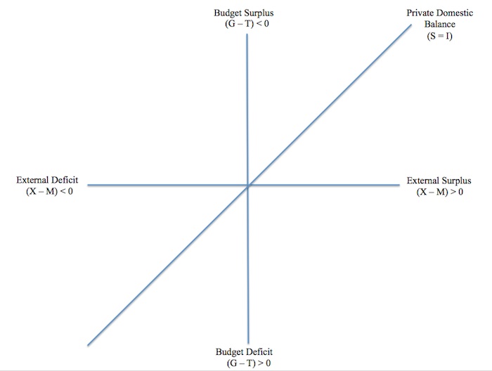
From Equation (6.4) we learned that the sum of the sectoral balances is zero as a matter of accounting – so (I – S) + (G – T) + (X – M) = 0. Imagine that we construct an axis defining four quadrants. Figure 6.7 depicts the Budget balance on the vertical axis and the external balance on the horizontal axis.

So all points above zero on the vertical axis represent a budget surplus (G < T) and all points below zero on the vertical axis denote budget deficits (G > T).

Similarly, all points to the right of the zero line on the horizontal axis denote external surpluses (X > M) and all points to the left of zero on the horizontal axis represent external deficits (X < M). Clearly, the origin of the axis denotes a position where all balances are equal to zero. From the insight gained from Equation (6.4), we also know that when the Private Domestic Balance is zero (S = I), then the Budget deficit (surplus) has to equal the External deficit (surplus). From Figure 6.7, the diagonal 45⁰ line thus shows all combinations of budget and external balances where the Private Domestic Balance is zero (S = I). We will refer to this as the SI line.

Figure 6.7 A Graphical Sectoral Balances Framework

Source: DOCUMENT SOURCE

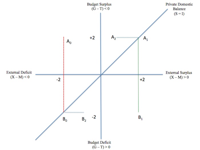
We can use that knowledge to determine the segments of the diagram where the Private Domestic Balance is in surplus (S > I) and in deficit (S < I). To make it easier, we can express the Sectoral Balances Equation (6.4) in a different way: (6.6)      (S - I) = (G - T) + (X - M) Equation (6.6) is just another way of expressing the accounting rule but in this case isolates the Private Domestic Balance on the left-hand side. Consider the red dotted-line A₀B₀ in Figure 6.7a, which cuts the horizontal axis where the External deficit is 2 per cent of GDP. All points on that line segment correspond to a Budget deficit of less than 2 per cent of GDP or a Budget surplus depending on which side of the horizontal axis we are considering.

The Private sector is in balance only at Point B₀ where the budget deficit equals the external deficit. So all points along A₀B₀ correspond to Private Domestic deficits (S < I). Now consider the green dotted-line A₁B₁, which cuts the horizontal axis where the External surplus is 2 per cent of GDP. All points on that line segment correspond to a Budget surplus of less than 2 per cent of GDP or a Budget deficit depending on which side of the horizontal axis we are considering.

The Private sector is in balance only at Point A₁ where the budget surplus equals the external surplus. So all points along A₁B₁ correspond to Private Domestic surpluses (S > I).

Now consider the blue dotted-line A₁A₂. At Point A₁, the Private sector is in balance because the budget surplus equals the external surplus.

Moving along A₁A₂ we encounter points where the external balance is less than the budget surplus and thus have to correspond to a Private Domestic deficit (S < I). Similarly, along B₀B₂, we move from a Private sector balance at B₀, to points where the external deficit is less than the budget deficit, which means the Private Domestic balance will be in surplus (S > I).

Figure 6.7a – Deriving the Private domestic sector balances

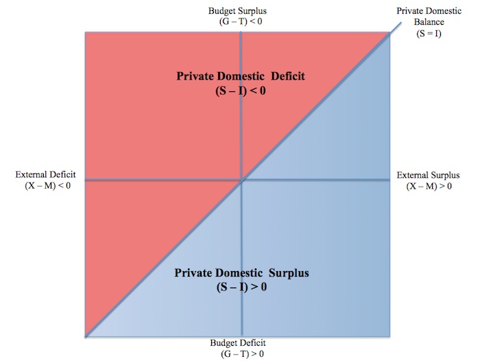
We can thus generalise this knowledge and conclude that all points above the 45⁰ line on either side of the vertical axis correspond to Private Domestic sector deficits and all points below the 45⁰ line on either side of the vertical axis correspond to Private Domestic sector surpluses.

Figure 6.7b renders this conclusion graphically.

Figure 6.7b Private domestic surpluses and deficits

This graphical framework thus allows us to examine the implications of different policy options.

For a sovereign, currency-issuing government any point in the four-quadrants is permissible. With private sector spending and saving decisions combining with the flows of income arising from trade with the external sector driving national income, the government sector can allow its balance to adjust to whatever magnitude is required to maintain full employment and price stability.

For example, if the external account was in deficit and the private sector was saving overall, then the drain on aggregate demand would require the government to run a deficit of sufficient size to ensure total spending was sufficient to absorb the real productive capacity available in the economy.

Alternatively, the external sector might be in surplus which would add to aggregate demand while the private sector might spending more than it is earning, that is, in deficit overall. In these situations the government would have to ensure it ran a surplus of sufficient size to ensure the economy did not overheat and exhaust its productive capacity.

The strong economy would be associated with robust tax revenue growth, which would help the government achieve its surplus. But discretionary adjustments in spending and taxation rates might also be required.

But while any point would be permissible, we know that the private sector cannot sustain deficits permanently. This is because the flows of spending which deliver deficits have to be funded. As we learned in the earlier section of this Chapter when we considered the flow of funds, private deficits ultimately manifest in an increasing stock of debt being held on the private sector’s balance sheet.

This process of debt accumulation is finite in capacity because at some point the susceptibility of the balance sheet to cyclical movements (for example, rising unemployment) rises and the risk of default increases. In some historical instances, this process has collapsed after serious debt defaults occurred (for example, in the early months of the Global Financial Crisis in 2007-08). In other times, the private sector starts to reduce the precariousness of its balance sheet by reducing spending and increasing saving in order to bring the debt levels it is carrying down to more sustainable levels.

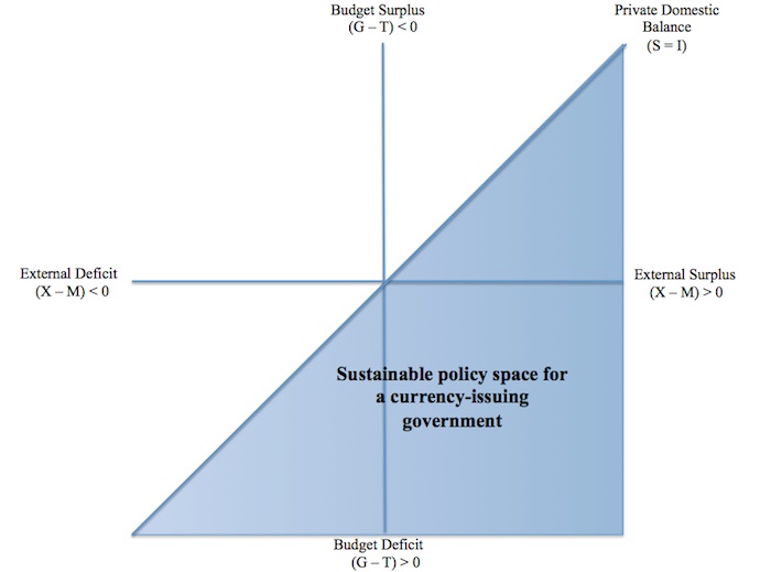
In the long-term, the only sustainable position is for the private domestic sector to be in surplus. An economy can absorb deviations around that position but only for short-periods.

[NOTE: The following reflects the analysis presented by Avraham Baranes and Stephanie Kelton University – Bird Brains:From Austerity to Prosperity A Guided Tour Through the Deficit Aviary – at the 11th International Post Keynesian Conference Kansas City, September 2012]

Figure 6.8 shows what we might define as the sustainable space available to governments that issue their own currency.

Figure 6.8 Sustainable space for sovereign governments

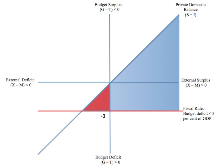
Now imagine that the government is forced to operate under a fiscal rule that bans budget deficits greater than 3 per cent of GDP as shown by the red line in Figure 6.9. In Chapter 18 we will consider the so-called Eurozone crisis. We will learn that the formation of the common monetary union introduced just such a fiscal rule under its Stability and Growth Pact. The aim was to restrict the capacity of each member state to run deficits.

While our discussion in Chapter 18 will embrace the wider political economic debates about the imposition of that fiscal rule, for now, consider what it means for both permissible and sustainable spaces available to a macroeconomic policy maker.

Clearly any point above the 3 per cent of GDP budget deficit rule is permissible. However, using the same logic as before, the sustainable space requires that the private domestic sector be in surplus overall, even though short-term deviations from this status can occur from time to time.

Figure 6.9 shows the sustainable space for such an economy (the combination of red and blue areas). The blue-shaded areas shows the sustainable space available to policy makers in nations that run external surpluses. The red-shaded areas shows the sustainable space available to policy makers in nations that run external deficits.

Thus the policy space that governments have to operate within when fiscal rules are imposed is very limited relative to the options available to a sovereign, currency-issuing government, which operates without any direct quantitative restrictions on the deficits they can run.

Figure 6.9 Sustainable space for governments constrained by fiscal rules

Why is this important? A rule-free government can always utilise the available space to ensure aggregate demand is sufficient to maintain full employment and price stability.

By definition, not every nation can run an external surplus because a surplus has to be matched by a deficit or deficits in other nations. While the external surplus nations have more policy flexibility when operating under a fiscal rule, of the type shown in Figure 6.9, it still remains that the allowable budget deficits may be in sufficient to maintain sufficient aggregate demand necessary to sustain full employment.

The policy inflexibility facing nations which run external deficits and simultaneously have to operate under fiscal rules as shown in Figure 6.9 become even more restrictive. When such an economy experiences a negative economic shock which leads the private sector to seek to reduce its spending and target sectoral surpluses, the extent to which the budget deficit can move to absorb the loss of overall aggregate demand is very limited.

It is highly likely that such an economy will experience enduring recessions as a result of the artificial fiscal rules (restrictions) that are placed on the government.

The sustainable goal for a government should be to maintain full employment and price stability and allow its budget balance to adjust accordingly to ensure aggregate demand is consistent with that goals. A sovereign, currency-issuing government can always meet those goals if it chooses.

However, the imposition of fiscal rules restricts the government from achieving these goals and makes the budget deficit the goal rather than the more significant macroeconomic goals of full employment and price stability.

The lesson is that the government should never specifically target any particular budget outcome, but, rather, should target employment growth and price level stability.

Conclusion

Next week I will move on to the Chapter on Trade (I think).

Saturday Quiz

The Saturday Quiz will be back again tomorrow. It will be of an appropriate order of difficulty (-:

That is enough for today!

(c) Copyright 2012 Bill Mitchell. All Rights Reserved.