Aggregate Demand – part 7 (final)

I am now using Friday’s blog space to provide draft versions of the Modern Monetary Theory textbook that I am writing with my colleague and friend Randy Wray. We expect to complete the text by the end of this year. Comments are always welcome. Remember this is a textbook aimed at undergraduate students and so the writing will be different from my usual blog free-for-all. Note also that the text I post is just the work I am doing by way of the first draft so the material posted will not represent the complete text. Further it will change once the two of us have edited it.

[NOTE: The redux notation in the title refers to re-edits of earlier blogs with the same title. At present, the updated Chapter starts from Aggregate demand – Part 5 (redux) and continues today. Earlier Parts in the Aggregate Demand series are redundant and should be ignored].

[RESUMING FROM LAST WEEK’s ANALYSIS – Aggregate demand – Part 6 (redux)]

What happens if autonomous spending changes?

In Figure 8.6 we learned that if any of the components of autonomous aggregate expenditure changes, the Aggregate Demand Function shifts up or down, with the extent of the shift being measured by the change in the vertical intercept.

Assume that government spending rises as a result of the government being concerned that the rate of unemployment is too high. In Chapter 10, we will learn that mass unemployment is always the result of deficient aggregate demand relative to the productive potential of the economy and a simple remedy is for governments to increase total spending.

Figure 8.10 shows the change in equilibrium expenditure and income when government spending increases (ΔG). Point A is the initial equilibrium real GDP and national income level, Y*₀, which corresponds to aggregate expenditure of E*₀. The Aggregate Demand Function is given as E = C + I + G₀ + NX).

At this point there are no unplanned inventory changes and firms are production decisions based upon there expected aggregate demand are being realised.

Now government spending increases by ΔG, which increases the Aggregate Demand Function (such that E = C + I + G₁ + NX) and real GDP and national income increases to Y*₁, which corresponds to aggregate expenditure of E*₁. The new equilibrium national income is at Point B.

The reason that equilibrium real GDP and national income increases relates to the firms revision of expected expenditure. When the government injects the new autonomous spending in to the economy, aggregate spending at the current equilibrium is greater than real Output. The difference is the line segment AA’.

This distance indicates the excess aggregate demand (relative to current real GDP) and inventories would be becoming depleted. Firms would soon revise their expectations of aggregate demand upwards and start to produce more real output and pay out higher levels of national income.

They would continue to increase production and national income until their aggregate demand expectations were consistent with actual aggregate demand, a state which occurs at Point B (where the new Aggregate Demand Function cuts the 45⁰ aggregate supply line).

Note that the change in equilibrium national income, ΔY is greater than the initial change in autonomous expenditure, ΔG. The difference between the two changes is given by the line segment CD.

How do we explain this difference?

The expenditure multiplier indicates by how much real GDP and national income changes when there is a change in autonomous expenditure. The larger is the multiplier, the larger is the change in real GDP and national income for a given change in autonomous expenditure.

The total change in aggregate demand (ΔE) following a change in autonomous expenditure (in this case, ΔG) is the sum of ΔG and the induced consumption spending that follows the initial rise in national income. Refer back to Figure 8.9 if you are unsure about this point.

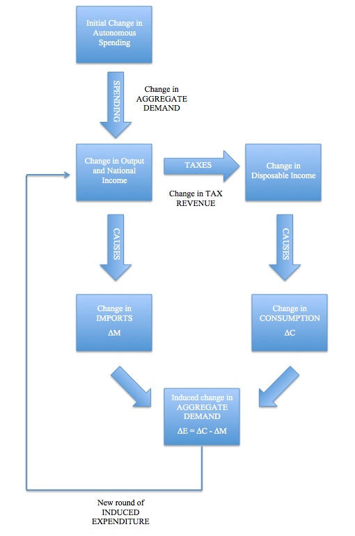
The induced consumption spending is the lower chain of events in Figure 8.9. As firms react to the initial disequilibrium at Point A (the excess aggregate demand AA’) by increasing real GDP and national income, households, in turn, increase their consumption expenditure. But at the same time, imports are rising by mΔY, tax revenue is rising by tΔY, and households save a portion of each extra dollar of disposable income, (1-c)ΔYd.

These leakages mean that each subsequent round of induced spending is smaller than the last and eventually become zero. At that point, the economy reaches the new equilibrium at Point B in Figure 8.10.

So the total change in real output and national income, ΔY is equal to the total change in aggregate expenditure, ΔE, which is equal to the initial change in autonomous spending, ΔA plus the induced consumption ΔC.

Figure 8.11 provides a flow diagram of the sequence of events that see an initial rise in autonomous expenditure multiply through the expenditure system, with leakages at each stage of the induced spending.

Figure 8.11 The multiplier flow map

Numerical example of the expenditure multiplier at work

Imagine that the marginal propensity to consume (c) is 0.80, the current tax rate is 0.20, and the marginal propensity to import is 0.20. This means that for every dollar of national income produced:

• 20 cents goes to tax revenue and is drained from the domestic economy.
• Disposable income thus rises by 80 cents and household consumption rises by 64 cents with the residual being increased saving of 16 cents.
• In turn, for every subsequent dollar of disposable income generated after taxes are taken out, households consume 80 cents and save 20 cents.
• 20 cents goes into new import expenditure and is lost to the domestic
• Total leakages from every extra dollar generated are thus 56 cents.

The way to think of the second-round expenditure injection is to focus on the leakages. After taxation is taken out, consumers determine how much they wish to spend on increased consumption, with saving then being the residual that drains further demand.

But as a result of the higher national income, total imports have also risen by 20 cents in the dollar and so the actual new spending that occurs is the difference between consumption spending and imports, which in this example is 44 cents.

Refer back to Figure 8.11 to reinforce your understanding of the sequence of events.

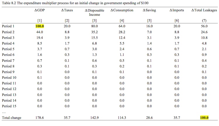
Table 8.2 shows the process for 15 periods (by which the induced consumption is near zero) and the final change in income that results from the initial rise in government spending by $100. In the on-line resources available for this Chapter on the support page, you will be able to download the spreadsheet and manipulate the initial expenditure injection, the tax rate and the marginal propensity to consume to produce your own simulations.

In the example shown, the extra $100 in government spending, leads firms to produce more output and increase income payments by $100 (under the assumptions in this Chapter that firms are quantity adjusters).

Already you can understand that the initial spending increase of $100, which might have been a government order for new public school buildings, provides workers involved in the production of those buildings with increased incomes. These workers, then spend some of their income gains on various goods and services (for example, local shops, local service suppliers, goods and services from firms not in their local area etc).

Taxes rise by $20 (0.20 x $100) leaving a rise in disposable income of $80. Households increase their consumption in Period 1 by $64 (0.8 x $80) and save the residual of the increase in disposable income, $16.

The economy also loses $20 dollars of expenditure to imports (0.2 x $100).

The induced increase in expenditure in Period 2 is thus the extra consumption ($64) less the leakage from the imports ($20) which is $44. That induced expenditure increase stimulate further income and production and the multiplier adjustment process is underway.

Each successive induced spending increase is smaller than the last because of the leakages.

The initial spending “fans out” or spreads throughout the entire economy. The initial spending multiplies into a much larger increase in spending.

Note the Leakages are getting smaller with each spending period following the initial injection of $100. In the bottom row we see that the sum of all the period-by-period changes in GDP (Column [1]) equals $178. The total increase in tax revenue (Column [2]) is $35.70. The total increase in disposable income (Column [3]) is thus $142.90, which leads to total induced consumption (Column [4]) of $114.3 and the total increase in saving (Column [5]) is $28.60. Total Imports (Column [6]) rise by $35.70.

The total leakages from the expenditure system – taxes, saving and imports – sum to $100.00 at the end of the adjustment period, which is the amount of the total initial injection in autonomous expenditure. At the point when leakages equal the injections, the system is at rest and the multiplied impact of the initial injection in autonomous expenditure is complete.

Think back to our algebraic definition of national income equilibrium shown in Equation (8.16) and the related expression for the expenditure multiplier, Equation (8.17).

If we substitute the assumed values in this example into the multiplier formula we get:

multiplier = ΔY/ΔG = 1/[1 – c(1 – t) + m] = 1/[1 – 0.8(1 – 0.20) + 0.20] = 1.785

The multiplier is the total change in GDP for a one dollar initial increase in aggregate demand. In this example, given the values of the marginal propensity to consume, the tax rate and the marginal propensity to import) the multiplier is calculated to be 1.785 (rounded).

That means, that if autonomous expenditure (for example, government spending) rose by $100, the total change in GDP, after the economy adjusts to the higher production and income levels, would be $178.50 (rounded).

Changes in the magnitude of the expenditure multiplier

Equation (8.17) defined the expenditure multiplier as ΔY/ΔG = 1/[1 – c(1 – t) + m], which means that its size depends on the marginal propensity to consume (c), the tax rate (t) and the marginal propensity to import (m).

The following conclusions can be drawn at this stage:

• The multiplier is larger (smaller) the larger (smaller) is the marginal propensity to consume (c).
• The multiplier is larger (smaller) the smaller (larger) is the marginal propensity to import (m). The more open the economy to trade, the lower is multiplier.
• The multiplier is larger (smaller) the smaller (larger) is the tax rate (t).

A higher marginal propensity to consume means that each successive round of induced consumption spending is larger, other things equal. Given that the marginal propensity to save (s) is just (1-c), the multiplier is higher when the marginal propensity to save is lower.

In general, the lower are the leakages (taxes, saving and imports) from the expenditure system, the higher will be multiplier. This is because the lower the leakages from each spending round, the larger is the induced consumption and the longer is the adjustment process following an initial injection of demand.

What happens if households decide to save more per dollar of disposable income received? That is, what will be the impact on national income and output if the marginal propensity to consume falls?

Earlier in the Chapter, we learned that the slope of the Aggregate Demand Function (see Figure 8.5) was [c(1-t) – m], which tells us that the change in aggregate spending for a given change in national income is larger, the larger is the marginal propensity to consume (c) and the lower is the tax rate (t) and the marginal propensity to import (m).

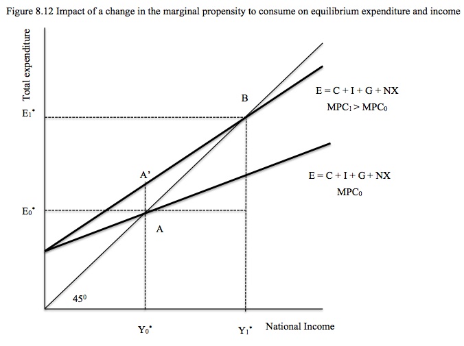
Consider an increase in the marginal propensity to consume (c). Figure 8.12 depicts this case. The initial Aggregate Demand Function (for MPC₀) is associated with a national income equilibrium at Point A where E*₀ generates production and national income of Y*₀.

When the marginal propensity to consume rises to MPC₁, the Aggregate Demand Function pivots upwards at the vertical intercept. At the current equilibrium income level, Y*₀, households choose to spend an increased proportion of each dollar of disposable income on consumption. The initial change in aggregate demand (E) is measured by the distance A to A’.

The economy responds to the increased consumption spending by increasing production and national income. The higher multiplier (as a result of the higher MPC) then drives national income up further and the economy reaches a new equilibrium at Point B. At that point the economy comes to rest again.

The following conclusions can be drawn at this stage:

• The slope of the Aggregate Demand Function is steeper (shallower) the larger (smaller) is the marginal propensity to consume (c). This means that for a given flow of autonomous spending, aggregate demand and national income will be higher if the marginal propensity to consume rises, and vice versa.
• The slope of the Aggregate Demand Function is steeper (shallower) the smaller (larger) is the marginal propensity to import (m). This means that for a given flow of autonomous spending, aggregate demand and national income will be higher if the marginal propensity to import falls, and vice versa.
• The slope of the Aggregate Demand Function is steeper (shallower) the smaller (larger) is the tax rate (t). This means that for a given flow of autonomous spending, aggregate demand and national income will be higher if the tax rate falls, and vice versa.

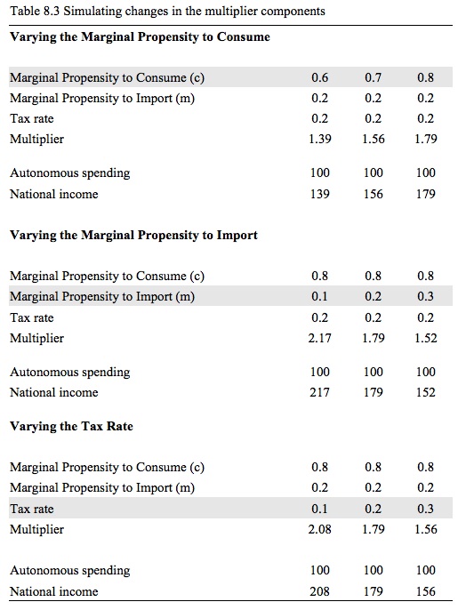
Table 8.3 shows the impact of varying the parameters that determine the size of the multiplier (c, m and t) on national income for a given injection of autonomous expenditure. You might like to simulate multiple changes in the parameters (for example, a rising MPC and a rising tax rate) to gain a greater understanding of how these influences interact.

[A FINAL SECTION WILL FOLLOW HERE]

[THEN THERE WILL BE A SUMMARY OF THE MAJOR POINTS IN THE CHAPTER BY WAY OF CONCLUSION]

Conclusion

This Chapter is now more or less drafted (noting the last sections still to be added) and we will turn to editorial issues (including all those raised by the comments – for which I am appreciative).

Next week, I plan to move onto the chapter on Sectoral Balances (Chapter 6), which in the sequence follows the Chapter on National Accounting. The next chapter after NIPA is Chapter 8 Introduction to effective demand – D-Z nominal, and then the Chapter on Aggregate Demand, covered in the last several Friday blogs.

Saturday Quiz

The Saturday Quiz will be back again tomorrow. It will be of an appropriate order of difficulty (-:

That is enough for today!

(c) Copyright 2012 Bill Mitchell. All Rights Reserved.