Aggregate demand – Part 5 (redux)

I am now using Friday’s blog space to provide draft versions of the Modern Monetary Theory textbook that I am writing with my colleague and friend Randy Wray. We expect to complete the text by the end of this year. Comments are always welcome. Remember this is a textbook aimed at undergraduate students and so the writing will be different from my usual blog free-for-all. Note also that the text I post is just the work I am doing by way of the first draft so the material posted will not represent the complete text. Further it will change once the two of us have edited it.

Please read this blog as a continuation of last week’s – Aggregate demand – Part 4 (redux) – which sought to consolidate the edits to date on this Chapter’s material.

[WE PICK UP WHERE WE LEFT OFF LAST TIME]

We can use the techniques you learned in Chapter 4 to modify Equation (8.12).

(8.13)      E = C₀ + I + G + X + [c(1 – t) – m]Y

We could usefully simplify this expression by collection all the components of total expenditure that are autonomous (such that A = C₀ + I + G + X) to write the Aggregate Demand Function as:

(8.14)      E = A + [c(1 – t) – m]Y

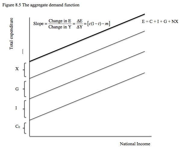
The slope of this function – ΔE/ΔY = [c(1 – t) – m] – which tells us that the change in aggregate spending for a given change in national income is larger, the larger is the marginal propensity to consume (c) and the lower is the tax rate (t) and the marginal propensity to import (m).

See if you can explain this result to yourself at this point. Think about the marginal propensity to consume as leading to an induced consumption expenditure increase when national income rises and the tax rate and marginal propensity to import being leakages from the expenditure system for each dollar rise in national income. We will provide a full analysis of this in the next section when we consider the expenditure multiplier.

Figure 8.5 shows the Aggregate Demand Function and its individual components. We add all the autonomous expenditure items to get the intercept of the function.

The Aggregate Demand Function is drawn with national output/income on the horizontal axis and aggregate demand or planned expenditure on the vertical axis.

It shows the relationship between between national income and planned expenditure and two aspects are important:

• Total autonomous spending – the horizontal intercept; and
• The slope of the function which depends on the marginal propensity to consume (c), the marginal propensity to import (m) and the tax rate (t). and the marginal propensity to import (m).

Aggregate demand (planned expenditure) will change at every level of national income if any of the components that make up autonomous spending or the slope changes.

Referring to Figure 8.5, if planned government spending or private investment was to rise, then the Aggregate Demand Function would shift upwards – the vertical intercept would rise by the rise in planned spending. As a result, planned spending would be higher at each income level. The opposite would be the case if, for example, government spending was cut.

Figure 8.6 shows the impact of a rise in autonomous spending from A₀ to A₁.

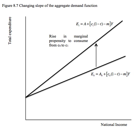
The Aggregate Demand Function may also change its slope. A rise in the marginal propensity to consume (c) and/or a fall in the tax rate (t) and/or the marginal propensity to import (m) will increase the slope of the function.

Figure 8.7 shows the impact of a rise in the marginal propensity to consume (c). At every national income level, planned spending is now higher.

See if you can sketch the impacts and explain the meaning of a rise in the tax rate (t), a rise in the marginal propensity to import (m) and a fall in the marginal propensity to consume (c).

You should also try to articulate what factors will influence the actual values of the marginal propensity to consume (c) and marginal propensity to import (m) in the real world. For example, poorer nations with basic financial systems might be expected to have a higher marginal propensity to consume than nations with high disposable income and widespread access to credit.

Equilibrium national income

The term equilibrium in macroeconomics is used to refer to a situation where there are no forces present which would alter the current level of spending, output and national income. At that point, firms are selling all the output they produced based on their expectations of planned expenditure.

You should be very careful not to confuse equilibrium with full employment. A macroeconomic equilibrium can occur at times when there is very high involuntary unemployment as we will learn in Chapter 10. Full employment is only one possible point of equilibrium.

Equilibrium occurs when planned expenditure is equal to national income and output.

Under our current assumption that firms in the economy are quantity-adjusters and prices are fixed in the short-term, Figure 8.1 showed us that the 45⁰ line was the aggregate supply curve. At each point the firms are realising their expectations and ratifying their decision to supply real output to the market. The ratification comes through the receipt of expected income that covers both their costs in aggregate and the desired volume of profits.

We are implicitly assuming that there are idle resources available for firms to deploy in expanding output. At some point, when the economy is operating at full capacity, firms are unable to continue expanding real output in response to additional spending. At that point, price rises are inevitable.

Equilibrium thus occurs when the Aggregate Demand Function cuts the 45⁰ line for at this point, the aggregate demand expectations formed by the firms, which motivated their decisions to supply – Y^* – are consistent with the planned expenditure – E^* – by consumers, firms, government and the external economy.

Figure 8.8 shows the equilibrium income (Y^*) and expenditure (E^*) combination. In terms of the terminology used in Chapter 7, this point defines the effective demand in the economy at this point in time.

Note the two areas that lie between the Aggregate Demand Function and the 45⁰ line. The area A (Zone A) is characterised by planned expenditure being greater than expected demand and hence actual output and income. Firms have undersupplied output and generated less national income than would be consistent with actual planned expenditure.

In this situation, unplanned inventory run-down provides the signal to firms that they have been mistaken in their expectations. Firms would react to this unplanned run-down in inventories by increasing output and national income.

Similarly, the area B (Zone B) is characterised by planned expenditure being less than expected demand and hence actual output and income. Firms have been too optimistic and over-supplied output and generated more national income than would be consistent with actual planned expenditure.

In this situation, unplanned inventory build-up provides the signal to firms that they have been mistaken in their expectations. Firms would react to this unplanned build-up in inventories by decreasing output and national income.

The inventory cycle is an important part of the cyclical adjustments that quantity-adjusting firms make to bring their expectations and production decisions into line with planned expenditure.

The importance of the inventory cycle is that they lead to changes in production and income which bring the economy back into equilibrium. The decision to increase production means that more employment will be created and the higher national income leads to an increase in planned expenditure.

Firms will continue increasing output, income and employment until their expectations are matched by planned expenditure and there are no further unplanned reductions in inventories. Equilibrium is reached at the Y*-E* combination, that is, where the Aggregate Demand Function cuts the 45⁰ Aggregate Supply line.

Similarly, firms will continue decreasing output, income and employment until there are no further unplanned increases in inventories. Once again the income adjustments bring the economy back to the Y*-E* combination. At that point, planned inventories are being held and firms are producing exactly as much as planned expenditure.

The Expenditure Multiplier

There is an additional feature of this income adjustment mechanism that is important to understand. In the Aggregate Demand Function (Equation 8.14) you can see that total planned expenditure is composed of two components: (a) the autonomous spending component (A = C₀ + I + G + X); and (b) expenditure induced by the level of national income, [c(1 – t) – m]Y.

What would be the impact on real GDP (and national income) if one of the components of autonomous spending changed? We know that real GDP and national income will rise if planned spending rose and will fall if planned spending falls. The question of interest now is by how much will real GDP and national income change after a change in planned spending driven by a change in autonomous spending (for example, an increase in govermment spending).

Economists have developed the concept of the expenditure multiplier to estimate how much national income (Y) will change for a given change in autonomous spending (A).

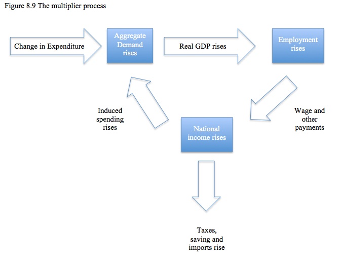
Figure 8.9 sketches the expenditure multiplier process. From an initial equilibrium position, a change in autonomous expenditure provides an instant boost to aggregate demand. Firms respond to the increased planned expenditure as explained in the last section and increase employment to produce the increased real GDP. Wage and payments to other inputs increase which sum to an increase in national income.

The rise in national income induces further consumption spending which leads to a rise in aggregate demand. A proportion of the rise in national income leaks out in the form of higher tax payments, rising imports and increased saving.

The process continues until the induced spending becomes so small that there is no further real GDP increases. The process works in reverse for a fall in autonomous expenditure.

The formal expression for the expenditure multiplier is derived directly from the equilibrium national income and expenditure relationship.

The Aggregate Demand Function was given as E = A + [c(1 – t) – m]Y. The national income equilibrium condition is given as:

(8.15)      Y = E

If we substitute the equilibrium condition into the Aggregate Demand Function (8.14) we get:

(8.16a)      Y = E = A + [c(1 – t) – m]Y

And solving for Y (collecting Y terms on left-hand side) gives:

(8.16b)      Y[1 – c(1 – t) + m] = A

Thus equilibrium income is:

(8.16)      Y = 1/[1 – c(1 – t) + m]A

The expenditure multiplier (α) is the coefficient next to the A term in Equation (8.16):

(8.17)      α = ΔE/ΔY = 1/[1 – c(1 – t) + m]

So if A changes by $1 then Y changes by 1/[1 – c(1 – t) + m] or α times the change in A.

By inspecting the terms that define the expenditure multiplier, you can see that it is a ratio involving the marginal propensity to consume (c), the marginal tax rate (t) and the marginal propensity to import.

Applying the tools you learned in Chapter 4, you can observe the following things:

• Other things equal, the higher is the marginal propensity to consume the higher is the expenditure multiplier.
• Other things equal, the lower is the tax rate the higher is the expenditure multiplier.
• Other things equal, the lower is the marginal propensity to import, the higher is the expenditure multiplier.
• The opposite is the case if c is lower and t and m are higher.

The task now is to explain the economic processes that lead to these conclusions.

We start with the essential insight that aggregate demand drives output with generates incomes (via payments to the productive inputs). Accordingly, what is spent will generate income in that period which is then available for use. For example, workers who are hired by firms to produce goods and services spend the incomes they earn as do suppliers of raw materials and other inputs to the production process.

There are various ways in which the income derived from the payments arising from output production can be used. The income can be used for:

• Increased consumption.
• Increased saving.
• Relinquishing tax obligations to government.
• Increased import spending.

Conclusion

Net week I will finish this chapter by analysis changes in the multiplier and equilibrium income.

Saturday Quiz

The Saturday Quiz will be back again tomorrow. It will be of an appropriate order of difficulty (-:

That is enough for today!

(c) Copyright 2012 Bill Mitchell. All Rights Reserved.